Decomposition#

Decomposition techniques are most commonly used as a means of noise reduction (or denoising) and dimensionality reduction. To apply a decomposition to your dataset, run the decomposition() method, for example:

>>> s = hs.signals.Signal1D(np.random.randn(10, 10, 200))
>>> s.decomposition()
Decomposition info:
   normalize_poissonian_noise=False
   algorithm=SVD
   output_dimension=None
   centre=None

>>> # Load data from a file, then decompose
>>> s = hs.load("my_file.hspy")
>>> s.decomposition()

Note

The signal s must be multi-dimensional, i.e. s.axes_manager.navigation_size > 1

One of the most popular uses of decomposition() is data denoising. This is achieved by using a limited set of components to make a model of the original dataset, omitting the less significant components that ideally contain only noise.

To reconstruct your denoised or reduced model, run the get_decomposition_model() method. For example:

>>> # Use all components to reconstruct the model
>>> sc = s.get_decomposition_model()

>>> # Use first 3 components to reconstruct the model
>>> sc = s.get_decomposition_model(3)

>>> # Use components [0, 2] to reconstruct the model
>>> sc = s.get_decomposition_model([0, 2])

Sometimes, it is useful to examine the residuals between your original data and the decomposition model. You can easily calculate and display the residuals, since get_decomposition_model() returns a new object, which in the example above we have called sc:

>>> (s - sc).plot()

You can perform operations on this new object sc later. It is a copy of the original s object, except that the data has been replaced by the model constructed using the chosen components.

Controlling laziness of reconstructed models#

Both get_decomposition_model() and get_bss_model() accept a lazy_output keyword argument that controls whether the returned model is backed by a dask array:

lazy_output=None (default): return a lazy signal if the original signal is lazy, and an eager signal otherwise.
lazy_output=True: always return a lazy signal. This is useful when the reconstructed model is too large to keep in memory; you can call .save() afterwards to stream it to disk chunk by chunk.
lazy_output=False: always return an eager signal, computing the result immediately.

For lazy decomposition workflows, including svd_solver='full' and out-of-core saving, see Controlling laziness with the lazy_output keyword.

If you provide the output_dimension argument, which takes an integer value, the decomposition algorithm attempts to find the best approximation for the dataset \(X\) with only a limited set of factors \(A\) and loadings \(B\), such that \(X \approx A B^T\).

>>> s.decomposition(output_dimension=3)

Some of the algorithms described below require output_dimension to be provided.

Available algorithms#

HyperSpy implements a number of decomposition algorithms via the algorithm argument. The table below lists the algorithms that are currently available, and includes links to the appropriate documentation for more information on each one.

Note

Choosing which algorithm to use is likely to depend heavily on the nature of your dataset and the type of analysis you are trying to perform. We discuss some of the reasons for choosing one algorithm over another below, but would encourage you to do your own research as well. The scikit-learn documentation is a very good starting point.

Available decomposition algorithms in HyperSpy#
Algorithm	Method
“SVD” (default)	`svd_pca()`
“MLPCA”	`mlpca()`
“sklearn_pca”	`sklearn.decomposition.PCA`
“NMF”	`sklearn.decomposition.NMF`
“sparse_pca”	`sklearn.decomposition.SparsePCA`
“mini_batch_sparse_pca”	`sklearn.decomposition.MiniBatchSparsePCA`
“RPCA”	`rpca_godec()`
“ORPCA”	`orpca()`
“ORNMF”	`ornmf()`
custom object	An object implementing `fit()` and `transform()` methods (or `partial_fit()` for lazy signals; see Custom sklearn-like estimators)

Singular value decomposition (SVD)#

The default algorithm in HyperSpy is "SVD", which uses an approach called “singular value decomposition” to decompose the data in the form \(X = U \Sigma V^T\). The factors are given by \(U \Sigma\), and the loadings are given by \(V^T\). For more information, please read the method documentation for svd_pca().

>>> s = hs.signals.Signal1D(np.random.randn(10, 10, 200))
>>> s.decomposition()
 Decomposition info:
   normalize_poissonian_noise=False
   algorithm=SVD
   output_dimension=None
   centre=None

Note

In some fields, including electron microscopy, this approach of applying an SVD directly to the data \(X\) is often called PCA (see below).

However, in the classical definition of PCA, the SVD should be applied to data that has first been “centered” by subtracting the mean, i.e. \(\mathrm{SVD}(X - \bar X)\).

The "SVD" algorithm in HyperSpy does not apply this centering step by default. As a result, you may observe differences between the output of the "SVD" algorithm and, for example, sklearn.decomposition.PCA, which does apply centering.

Note

For lazy signals, the "SVD" algorithm supports additional parameters such as svd_solver ('randomized', 'incremental', or 'full') and centre. All three solvers support centre. See SVD (algorithm='SVD') for the full details.

Principal component analysis (PCA)#

One of the most popular decomposition methods is principal component analysis (PCA). To perform PCA on your dataset, run the decomposition() method with any of following arguments.

If you have scikit-learn installed:

>>> s.decomposition(algorithm="sklearn_pca")
 Decomposition info:
   normalize_poissonian_noise=False
   algorithm=sklearn_pca
   output_dimension=None
   centre=None
 scikit-learn estimator:
 PCA()

You can also turn on centering with the default "SVD" algorithm via the "centre" argument:

# Subtract the mean along the navigation axis
>>> s.decomposition(algorithm="SVD", centre="navigation")
 Decomposition info:
   normalize_poissonian_noise=False
   algorithm=SVD
   output_dimension=None
   centre=navigation

# Subtract the mean along the signal axis
>>> s.decomposition(algorithm="SVD", centre="signal")
 Decomposition info:
   normalize_poissonian_noise=False
   algorithm=SVD
   output_dimension=None
   centre=signal

You can also use sklearn.decomposition.PCA directly:

>>> from sklearn.decomposition import PCA
>>> s.decomposition(algorithm=PCA())
 Decomposition info:
   normalize_poissonian_noise=False
   algorithm=PCA()
   output_dimension=None
   centre=None
 scikit-learn estimator:
 PCA()

Poissonian noise#

Most of the standard decomposition algorithms assume that the noise of the data follows a Gaussian distribution (also known as “homoskedastic noise”). In cases where your data is instead corrupted by Poisson noise, HyperSpy can “normalize” the data by performing a scaling operation, which can greatly enhance the result. More details about the normalization procedure can be found in [Keenan2004].

To apply Poissonian noise normalization to your data:

>>> s.decomposition(normalize_poissonian_noise=True)

>>> # Because it is the first argument we could have simply written:
>>> s.decomposition(True)

Warning

Poisson noise normalization cannot be used in combination with data centering using the 'centre' argument. Attempting to do so will raise an error.

Maximum likelihood principal component analysis (MLPCA)#

Instead of applying Poisson noise normalization to your data, you can instead use an approach known as Maximum Likelihood PCA (MLPCA), which provides a more robust statistical treatment of non-Gaussian “heteroskedastic noise”.

>>> s.decomposition(algorithm="MLPCA")

For more information, please read the method documentation for mlpca().

Note

You must set the output_dimension when using MLPCA.

Robust principal component analysis (RPCA)#

PCA is known to be very sensitive to the presence of outliers in data. These outliers can be the result of missing or dead pixels, X-ray spikes, or very low count data. If one assumes a dataset, \(X\), to consist of a low-rank component \(L\) corrupted by a sparse error component \(S\), such that \(X=L+S\), then Robust PCA (RPCA) can be used to recover the low-rank component for subsequent processing [Candes2011].

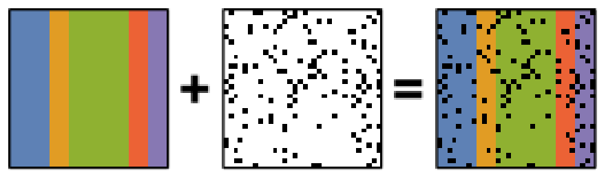
../../_images/rpca_schematic.png — Schematic diagram of the robust PCA problem, which combines a low-rank matrix with sparse errors. Robust PCA aims to decompose the matrix back into these two components.#

Note

You must set the output_dimension when using Robust PCA.

The default RPCA algorithm is GoDec [Zhou2011]. In HyperSpy it returns the factors and loadings of \(L\). RPCA solvers work by using regularization, in a similar manner to lasso or ridge regression, to enforce the low-rank constraint on the data. The low-rank regularization parameter, lambda1, defaults to 1/sqrt(n_features), but it is strongly recommended that you explore the behaviour of different values.

>>> s.decomposition(algorithm="RPCA", output_dimension=3, lambda1=0.1)
 Decomposition info:
   normalize_poissonian_noise=False
   algorithm=RPCA
   output_dimension=3
   centre=None

HyperSpy also implements an online algorithm for RPCA developed by Feng et al. [Feng2013]. This minimizes memory usage, making it suitable for large datasets, and can often be faster than the default algorithm.

>>> s.decomposition(algorithm="ORPCA", output_dimension=3)

The online RPCA implementation sets several default parameters that are usually suitable for most datasets, including the regularization parameter highlighted above. Again, it is strongly recommended that you explore the behaviour of these parameters. To further improve the convergence, you can “train” the algorithm with the first few samples of your dataset. For example, the following code will train ORPCA using the first 32 samples of the data.

>>> s.decomposition(algorithm="ORPCA", output_dimension=3, training_samples=32)

Finally, online RPCA includes two alternatives methods to the default block-coordinate descent solver, which can again improve both the convergence and speed of the algorithm. These are particularly useful for very large datasets.

The methods are based on stochastic gradient descent (SGD), and take an additional parameter to set the learning rate. The learning rate dictates the size of the steps taken by the gradient descent algorithm, and setting it too large can lead to oscillations that prevent the algorithm from finding the correct minima. Usually a value between 1 and 2 works well:

>>> s.decomposition(algorithm="ORPCA",
...                 output_dimension=3,
...                 method="SGD",
...                 subspace_learning_rate=1.1)

You can also use Momentum Stochastic Gradient Descent (MomentumSGD), which typically improves the convergence properties of stochastic gradient descent. This takes the further parameter subspace_momentum, which should be a fraction between 0 and 1.

>>> s.decomposition(algorithm="ORPCA",
...                 output_dimension=3,
...                 method="MomentumSGD",
...                 subspace_learning_rate=1.1,
...                 subspace_momentum=0.5)

Using the "SGD" or "MomentumSGD" methods enables the subspace, i.e. the underlying low-rank component, to be tracked as it changes with each sample update. The default method instead assumes a fixed, static subspace.

Note

The internal ORPCA class now provides a scikit-learn compatible API. If you use ORPCA directly (rather than through decomposition()), prefer the new methods:

partial_fit(X) — replaces the deprecated fit(X)
transform(X) — replaces the deprecated project(X)
components_ — replaces the deprecated finish()

The old methods still work but emit a VisibleDeprecationWarning and will be removed in a future release.

Non-negative matrix factorization (NMF)#

Another popular decomposition method is non-negative matrix factorization (NMF), which can be accessed in HyperSpy with:

>>> s.decomposition(algorithm="NMF")

Unlike PCA, NMF forces the components to be strictly non-negative, which can aid the physical interpretation of components for count data such as images, EELS or EDS. For an example of NMF in EELS processing, see [Nicoletti2013].

NMF takes the optional argument output_dimension, which determines the number of components to keep. Setting this to a small number is recommended to keep the computation time small. Often it is useful to run a PCA decomposition first and use the scree plot to determine a suitable value for output_dimension.

Note

For lazy signals, algorithm="NMF" is implemented via sklearn.decomposition.MiniBatchNMF (requires scikit-learn ≥ 1.1 for the out-of-core path; older versions fall back to in-memory sklearn.decomposition.NMF), which processes the data in chunks without loading the full dataset into memory. output_dimension is required in this case. See Machine learning for the full list of available lazy algorithms.

Robust non-negative matrix factorization (RNMF)#

In a similar manner to the online, robust methods that complement PCA above, HyperSpy includes an online robust NMF method. This is based on the OPGD (Online Proximal Gradient Descent) algorithm of [Zhao2016].

Note

You must set the output_dimension when using Robust NMF.

As before, you can control the regularization applied via the parameter “lambda1”:

>>> s.decomposition(algorithm="ORNMF", output_dimension=3, lambda1=0.1)

The MomentumSGD method is useful for scenarios where the subspace, i.e. the underlying low-rank component, is changing over time.

>>> s.decomposition(algorithm="ORNMF",
...                 output_dimension=3,
...                 method="MomentumSGD",
...                 subspace_learning_rate=1.1,
...                 subspace_momentum=0.5)

Both the default and MomentumSGD solvers assume an l2-norm minimization problem, which can still be sensitive to very heavily corrupted data. A more robust alternative is available, although it is typically much slower.

>>> s.decomposition(algorithm="ORNMF", output_dimension=3, method="RobustPGD")

Note

The internal ORNMF class now provides a scikit-learn compatible API. If you use ORNMF directly (rather than through decomposition()), prefer the new methods:

partial_fit(X) — replaces the deprecated fit(X)
transform(X) — replaces the deprecated project(X)
components_ — replaces the deprecated finish()

The old methods still work but emit a VisibleDeprecationWarning and will be removed in a future release.

Masks and reprojection#

Navigation and signal masks can be passed to decomposition() to restrict which pixels or channels are used during learning. Masked positions are excluded from the data matrix before the algorithm runs, and the resulting factors and loadings contain NaN at those positions by default.

>>> import numpy as np
>>> s = hs.signals.Signal1D(np.random.randn(10, 10, 200))

# Boolean array: True = exclude this navigation pixel
>>> nav_mask = np.zeros((10, 10), dtype=bool)
>>> nav_mask[0, :] = True   # mask the first row of navigation pixels

# Boolean array: True = exclude this signal channel
>>> sig_mask = np.zeros(200, dtype=bool)
>>> sig_mask[:10] = True    # mask the first 10 channels

>>> s.decomposition(
...     navigation_mask=nav_mask,
...     signal_mask=sig_mask,
... )

After decomposition the masked positions contain NaN:

learning_results.loadings has NaN rows for masked navigation pixels.
learning_results.factors has NaN rows for masked signal channels.

The reproject parameter can be used to fill those NaN positions by projecting the full (unmasked) data through the learned basis after learning is complete:

reproject='navigation': Projects all navigation pixels (including the masked ones) through the learned factors. This fills NaN in the loadings at masked navigation positions. Factors still contain NaN at masked signal channels.
reproject='signal': Projects all signal channels (including the masked ones) through the learned loadings via a pseudo-inverse. This fills NaN in the factors at masked signal channels. Loadings still contain NaN at masked navigation positions.
reproject='both': Applies both reprojections: factors and loadings are fully filled with no NaN remaining.

>>> s.decomposition(
...     navigation_mask=nav_mask,
...     signal_mask=sig_mask,
...     reproject="both",
... )

# loadings and factors both have no NaN after reproject='both'
>>> np.any(np.isnan(s.learning_results.loadings))
False
>>> np.any(np.isnan(s.learning_results.factors))
False

Note

For lazy signals, reproject='signal' and reproject='both' are supported for all algorithms, including "ORPCA" and "ORNMF", via the pseudo-inverse of the loadings. See Machine learning for more details.

Custom decomposition algorithms#

HyperSpy supports passing a custom decomposition algorithm, provided it follows the form of a scikit-learn estimator. Any object that implements fit and transform methods is acceptable, including sklearn.pipeline.Pipeline and sklearn.model_selection.GridSearchCV. You can access the fitted estimator by passing return_info=True.

>>> # Passing a custom decomposition algorithm
>>> from sklearn.preprocessing import MinMaxScaler
>>> from sklearn.pipeline import Pipeline
>>> from sklearn.decomposition import PCA

>>> pipe = Pipeline([("scaler", MinMaxScaler()), ("PCA", PCA())])
>>> out = s.decomposition(algorithm=pipe, return_info=True)
 Decomposition info:
   normalize_poissonian_noise=False
   algorithm=Pipeline(steps=[('scaler', MinMaxScaler()), ('PCA', PCA())])
   output_dimension=None
   centre=None
 scikit-learn estimator:
 Pipeline(steps=[('scaler', MinMaxScaler()), ('PCA', PCA())])

>>> out
Pipeline(steps=[('scaler', MinMaxScaler()), ('PCA', PCA())])