Axes handling#
Setting axis properties#
The axes are managed and stored by the AxesManager class
that is stored in the axes_manager attribute of
the signal class. The individual axes can be accessed by indexing the
AxesManager, e.g.:
>>> s = hs.signals.Signal1D(np.random.random((10, 20 , 100)))
>>> s
<Signal1D, title: , dimensions: (20, 10|100)>
>>> s.axes_manager
<Axes manager, axes: (20, 10|100)>
Navigation axes:
+-------------+------+-------+--------+-------+-------------+
|     Name    | size | index | offset | scale |    units    |
+-------------+------+-------+--------+-------+-------------+
| <undefined> |  20  |   0   |  0.0   |  1.0  | <undefined> |
| <undefined> |  10  |   0   |  0.0   |  1.0  | <undefined> |
+-------------+------+-------+--------+-------+-------------+
Signal axes:
+-------------+------+--------+-------+-------------+
|     Name    | size | offset | scale |    units    |
+-------------+------+--------+-------+-------------+
| <undefined> | 100  |  0.0   |  1.0  | <undefined> |
+-------------+------+--------+-------+-------------+
>>> s.axes_manager[0]
<Unnamed 0th axis, size: 20, index: 0>
The navigation axes come first, followed by the signal axes. Alternatively, it is possible to selectively access the navigation or signal dimensions:
>>> s.axes_manager.navigation_axes[1]
<Unnamed 1st axis, size: 10, index: 0>
>>> s.axes_manager.signal_axes[0]
<Unnamed 2nd axis, size: 100>
For the given example of two navigation and one signal dimensions, all the following commands will access the same axis:
>>> s.axes_manager[2]
<Unnamed 2nd axis, size: 100>
>>> s.axes_manager[-1]
<Unnamed 2nd axis, size: 100>
>>> s.axes_manager.signal_axes[0]
<Unnamed 2nd axis, size: 100>
The axis properties can be set by setting the BaseDataAxis
attributes, e.g.:
>>> s.axes_manager[0].name = "X"
>>> s.axes_manager[0]
<X axis, size: 20, index: 0>
Added in version 2.2: set() and get() methods for navigation_axes
and signal_axes.
It is also possible to set multiple attributes of multiple axes at once, using the set()
of the navigation_axes and signal_axes attributes.
The get() returns a dictionary of the attributes. For example:
>>> s.axes_manager.navigation_axes.set(name=("X", "Y"), offset=10, units="nm")
>>> s.axes_manager.navigation_axes.get("name", "offset", "units")
{"name" : ("X", "Y"), "offset" : (10, 10), "units" : ("nm", "nm")}
Once the name of an axis has been defined it is possible to request it by its name e.g.:
>>> s.axes_manager["X"]
<X axis, size: 20, index: 0>
>>> s.axes_manager["X"].scale = 0.2
>>> s.axes_manager["X"].units = "nm"
>>> s.axes_manager["X"].offset = 100
It is also possible to set the axes properties using a GUI by calling the
gui() method of the AxesManager
>>> s.axes_manager.gui()
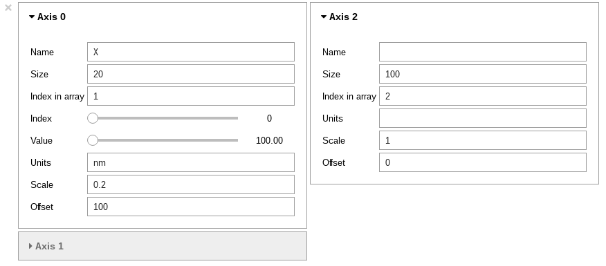
AxesManager ipywidgets GUI.#
or, for a specific axis, the respective method of e.g.
UniformDataAxis:
>>> s.axes_manager["X"].gui()
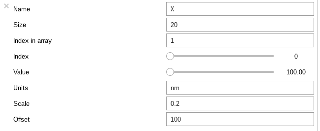
UniformDataAxis ipywidgets GUI.#
To simply change the “current position” (i.e. the indices of the navigation axes) you could use the navigation sliders:
>>> s.axes_manager.gui_navigation_sliders()
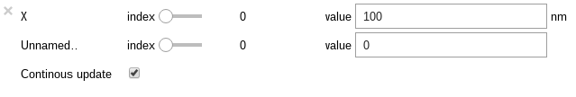
Navigation sliders ipywidgets GUI.#
Alternatively, the “current position” can be changed programmatically by
directly accessing the indices attribute of a signal’s
AxesManager or the index attribute of an individual
axis. This is particularly useful when trying to set
a specific location at which to initialize a model’s parameters to
sensible values before performing a fit over an entire spectrum image. The
indices must be provided as a tuple, with the same length as the number of
navigation dimensions:
>>> s.axes_manager.indices = (5, 4)
Summary of axis properties#
name(str) andunits(str) are basic parameters describing an axis used in plotting. The latter enables the conversion of units.navigate(bool) determines, whether it is a navigation axis.size(int) gives the number of elements in an axis.index(int) determines the “current position for a navigation axis andvalue(float) returns the value at this position.low_index(int) andhigh_index(int) are the first and last index.low_value(int) andhigh_value(int) are the smallest and largest value.The
axisarray stores the values of the axis points. However, depending on the type of axis, this array may be updated from the defining attributes as discussed in the following section.
Types of data axes#
HyperSpy supports different data axis types, which differ in how the axis is defined:
DataAxisdefined by an arrayaxis,FunctionalDataAxisdefined by a functionexpressionorUniformDataAxisdefined by the initial valueoffsetand spacingscale.
The main disambiguation is whether the
axis is uniform, where the data points are equidistantly spaced, or
non-uniform, where the spacing may vary. The latter can become important
when, e.g., a spectrum recorded over a wavelength axis is converted to a
wavenumber or energy scale, where the conversion is based on a 1/x
dependence so that the axis spacing of the new axis varies along the length
of the axis. Whether an axis is uniform or not can be queried through the
property is_uniform (bool) of the axis.
Every axis of a signal object may be of a different type. For example, it is common that the navigation axes would be uniform, while the signal axes are non-uniform.
When an axis is created, the type is automatically determined by the attributes passed to the generator. The three different axis types are summarized in the following table.
BaseDataAxis subclass |
Defining attributes |
|
|---|---|---|
axis |
False |
|
expression |
False |
|
offset, scale |
True |
Note
Not all features are implemented for non-uniform axes.
Warning
Non-uniform axes are in beta state and its API may change in a minor release. Not all hyperspy features are compatible with non-uniform axes and support will be added in future releases.
Uniform data axis#
The most common case is the UniformDataAxis. Here, the axis
is defined by the offset, scale and size parameters, which determine
the initial value, spacing and length, respectively. The actual axis
array is automatically calculated from these three values. The UniformDataAxis
is a special case of the FunctionalDataAxis defined by the function
scale * x + offset.
Sample dictionary for a UniformDataAxis:
>>> dict0 = {'offset': 300, 'scale': 1, 'size': 500}
>>> s = hs.signals.Signal1D(np.ones(500), axes=[dict0])
>>> s.axes_manager[0].get_axis_dictionary()
{'_type': 'UniformDataAxis', 'name': None, 'units': None, 'navigate': False, 'is_binned': False, 'size': 500, 'scale': 1.0, 'offset': 300.0}
Corresponding output of AxesManager:
>>> s.axes_manager
<Axes manager, axes: (|500)>
Signal axes:
+-------------+------+--------+-------+-------------+
|     Name    | size | offset | scale |    units    |
+-------------+------+--------+-------+-------------+
| <undefined> | 500  | 300.0  |  1.0  | <undefined> |
+-------------+------+--------+-------+-------------+
Functional data axis#
Alternatively, a FunctionalDataAxis is defined based on an
expression that is evaluated to yield the axis points. The expression
is a function defined as a string using the
SymPy text expression
format. An example would be expression = a / x + b. Any variables in the
expression, in this case a and b must be defined as additional
attributes of the axis. The property is_uniform is automatically set to
False.
x itself is an instance of BaseDataAxis. By default,
it will be a UniformDataAxis with offset = 0 and
scale = 1 of the given size. However, it can also be initialized with
custom offset and scale values. Alternatively, it can be a non
uniform DataAxis.
Sample dictionary for a FunctionalDataAxis:
>>> dict0 = {'expression': 'a / (x + 1) + b', 'a': 100, 'b': 10, 'size': 500}
>>> s = hs.signals.Signal1D(np.ones(500), axes=[dict0])
>>> s.axes_manager[0].get_axis_dictionary()
{'_type': 'FunctionalDataAxis', 'name': None, 'units': None, 'navigate': False, 'is_binned': False, 'expression': 'a / (x + 1) + b', 'size': 500, 'x': {'_type': 'UniformDataAxis', 'name': None, 'units': None, 'navigate': False, 'is_binned': False, 'size': 500, 'scale': 1.0, 'offset': 0.0}, 'a': 100, 'b': 10}
Corresponding output of AxesManager:
>>> s.axes_manager
<Axes manager, axes: (|500)>
Signal axes:
+-------------+------+-------------+-------------+-------------+
|     Name    | size |    offset   |    scale    |    units    |
+-------------+------+-------------+-------------+-------------+
| <undefined> | 500  | non-uniform | non-uniform | <undefined> |
+-------------+------+-------------+-------------+-------------+
Initializing x with offset and scale:
>>> from hyperspy.axes import UniformDataAxis
>>> dict0 = {'expression': 'a / x + b', 'a': 100, 'b': 10, 'x': UniformDataAxis(size=10,offset=10,scale=0.1)}
>>> s = hs.signals.Signal1D(np.ones(500), axes=[dict0])
>>> # the x array
>>> s.axes_manager[0].x.axis
array([10. , 10.1, 10.2, 10.3, 10.4, 10.5, 10.6, 10.7, 10.8, 10.9])
>>> # the actual axis array
>>> s.axes_manager[0].axis
array([20.        , 19.9009901 , 19.80392157, 19.70873786, 19.61538462,
   19.52380952, 19.43396226, 19.34579439, 19.25925926, 19.17431193])
Initializing x as non-uniform DataAxis:
>>> from hyperspy.axes import DataAxis
>>> dict0 = {'expression': 'a / x + b', 'a': 100, 'b': 10, 'x': DataAxis(axis=np.arange(1,10)**2)}
>>> s = hs.signals.Signal1D(np.ones(500), axes=[dict0])
>>> # the x array
>>> s.axes_manager[0].x.axis
array([ 1,  4,  9, 16, 25, 36, 49, 64, 81])
>>> # the actual axis array
>>> s.axes_manager[0].axis
array([110.        ,  35.        ,  21.11111111,  16.25      ,
        14.        ,  12.77777778,  12.04081633,  11.5625    ,
        11.2345679 ])
Initializing x with offset and scale:
(non-uniform) Data axis#
A DataAxis is the most flexible type of axis. The axis
points are directly given by an array named axis. As this can be any
array, the property is_uniform is automatically set to False.
Sample dictionary for a DataAxis:
>>> dict0 = {'axis': np.arange(12)**2}
>>> s = hs.signals.Signal1D(np.ones(12), axes=[dict0])
>>> s.axes_manager[0].get_axis_dictionary()
{'_type': 'DataAxis', 'name': None, 'units': None, 'navigate': False, 'is_binned': False, 'axis': array([  0,   1,   4,   9,  16,  25,  36,  49,  64,  81, 100, 121])}
Corresponding output of AxesManager:
>>> s.axes_manager
<Axes manager, axes: (|12)>
Signal axes:
+-------------+------+-------------+-------------+-------------+
|     Name    | size |    offset   |    scale    |    units    |
+-------------+------+-------------+-------------+-------------+
| <undefined> |  12  | non-uniform | non-uniform | <undefined> |
+-------------+------+-------------+-------------+-------------+
Defining a new axis#
An axis object can be created through the axes.create_axis() method, which
automatically determines the type of axis by the given attributes:
>>> from hyperspy import axes
>>> axis = axes.create_axis(offset=10,scale=0.5,size=20)
>>> axis
<Unnamed axis, size: 20>
Alternatively, the creator of the different types of axes can be called directly:
>>> from hyperspy import axes
>>> axis = axes.UniformDataAxis(offset=10,scale=0.5,size=20)
>>> axis
<Unnamed axis, size: 20>
The dictionary defining the axis is returned by the get_axis_dictionary()
method:
>>> axis.get_axis_dictionary()
{'_type': 'UniformDataAxis', 'name': None, 'units': None, 'navigate': False, 'is_binned': False, 'size': 20, 'scale': 0.5, 'offset': 10.0}
This dictionary can be used, for example, in the initilization of a new signal.
Adding/Removing axes to/from a signal#
Usually, the axes are directly added to a signal during signal
initialization. However, you may wish to add/remove
axes from the AxesManager of a signal.
Note that there is currently no consistency check whether a signal object has the right number of axes of the right dimensions. Most functions will however fail if you pass a signal object where the axes do not match the data dimensions and shape.
You can add a set of axes to the AxesManager by passing either a list of
axes dictionaries to axes_manager.create_axes():
>>> dict0 = {'offset': 300, 'scale': 1, 'size': 500}
>>> dict1 = {'axis': np.arange(12)**2}
>>> s.axes_manager.create_axes([dict0,dict1])
or a list of axes objects:
>>> from hyperspy.axes import UniformDataAxis, DataAxis
>>> axis0 = UniformDataAxis(offset=300,scale=1,size=500)
>>> axis1 = DataAxis(axis=np.arange(12)**2)
>>> s.axes_manager.create_axes([axis0,axis1])
Remove an axis from the AxesManager using remove(), e.g. for the last axis:
>>> s.axes_manager.remove(-1)
Using quantity and converting units#
The scale and the offset of each UniformDataAxis axis
can be set and retrieved as quantity.
>>> s = hs.signals.Signal1D(np.arange(10))
>>> s.axes_manager[0].scale_as_quantity
<Quantity(1.0, 'dimensionless')>
>>> s.axes_manager[0].scale_as_quantity = '2.5 µm'
>>> s.axes_manager
<Axes manager, axes: (|10)>
            Name |   size |  index |  offset |   scale |  units
================ | ====== | ====== | ======= | ======= | ======
---------------- | ------ | ------ | ------- | ------- | ------
     <undefined> |     10 |      0 |       0 |     2.5 |     µm
>>> s.axes_manager[0].offset_as_quantity = '2.5 nm'
Internally, HyperSpy uses the pint library to
manage the scale and offset quantities. The scale_as_quantity and
offset_as_quantity attributes return pint object:
>>> q = s.axes_manager[0].offset_as_quantity
>>> type(q) # q is a pint quantity object
<class 'pint.Quantity'>
>>> q
<Quantity(2.5, 'nanometer')>
The convert_units method of the AxesManager converts
units, which by default (no parameters provided) converts all axis units to an
optimal unit to avoid using too large or small numbers.
Each axis can also be converted individually using the convert_to_units
method of the UniformDataAxis:
>>> axis = hs.hyperspy.axes.UniformDataAxis(size=10, scale=0.1, offset=10, units='mm')
>>> axis.scale_as_quantity
<Quantity(0.1, 'millimeter')>
>>> axis.convert_to_units('µm')
>>> axis.scale_as_quantity
<Quantity(100.0, 'micrometer')>
Axes storage and ordering#
Note that HyperSpy rearranges the axes when compared to the array order. The following few paragraphs explain how and why.
Depending on how the array is arranged, some axes are faster to iterate than others. Consider an example of a book as the dataset in question. It is trivially simple to look at letters in a line, and then lines down the page, and finally pages in the whole book. However, if your words are written vertically, it can be inconvenient to read top-down (the lines are still horizontal, it’s just the meaning that’s vertical!). It is very time-consuming if every letter is on a different page, and for every word you have to turn 5-6 pages. Exactly the same idea applies here - in order to iterate through the data (most often for plotting, but for any other operation as well), you want to keep it ordered for “fast access”.
In Python (more explicitly numpy), the “fast axes order” is C order (also called row-major order). This means that the last axis of a numpy array is fastest to iterate over (i.e. the lines in the book). An alternative ordering convention is F order (column-major), where it is the other way round: the first axis of an array is the fastest to iterate over. In both cases, the further an axis is from the fast axis the slower it is to iterate over this axis. In the book analogy, you could think about reading the first lines of all pages, then the second and so on.
When data is acquired sequentially, it is usually stored in acquisition order.
When a dataset is loaded, HyperSpy generally stores it in memory in the same
order, which is good for the computer. However, HyperSpy will reorder and
classify the axes to make it easier for humans. Let’s imagine a single numpy
array that contains pictures of a scene acquired with different exposure times
on different days. In numpy, the array dimensions are (D, E, Y, X). This
order makes it fast to iterate over the images in the order in which they were
acquired. From a human point of view, this dataset is just a collection of
images, so HyperSpy first classifies the image axes (X and Y) as
signal axes and the remaining axes the navigation axes. Then it reverses
the order of each set of axes because many humans are used to get the X
axis first and, more generally, the axes in acquisition order from left to
right. So, the same axes in HyperSpy are displayed like this: (E, D | X,
Y).
Extending this to arbitrary dimensions, by default, we reverse the numpy axes, chop them into two chunks (signal and navigation), and then swap those chunks, at least when printing. As an example:
(a1, a2, a3, a4, a5, a6) # original (numpy)
(a6, a5, a4, a3, a2, a1) # reverse
(a6, a5) (a4, a3, a2, a1) # chop
(a4, a3, a2, a1) (a6, a5) # swap (HyperSpy)
In the background, HyperSpy also takes care of storing the data in memory in a “machine-friendly” way, so that iterating over the navigation axes is always fast.
Iterating over the AxesManager#
One can iterate over the AxesManager to produce indices to
the navigation axes. Each iteration will yield a new tuple of indices, sorted
according to the iteration path specified in iterpath.
Setting the indices property to a new index will
update the accompanying signal so that signal methods that operate at a specific
navigation index will now use that index, like s.plot().
>>> s = hs.signals.Signal1D(np.zeros((2,3,10)))
>>> s.axes_manager.iterpath # check current iteration path
'serpentine'
>>> for index in s.axes_manager:
...     print(index)
(0, 0)
(1, 0)
(2, 0)
(2, 1)
(1, 1)
(0, 1)
The iterpath attribute specifies the strategy that
the AxesManager should use to iterate over the navigation axes.
Two built-in strategies exist:
'serpentine'(default): starts at (0, 0), but when it reaches the final column (of index N), it continues from (1, N) along the next row, in the same way that a snake might slither, left and right.'flyback': starts at (0, 0), continues down the row until the final column, “flies back” to the first column, and continues from (1, 0).
>>> s = hs.signals.Signal1D(np.zeros((2,3,10)))
>>> s.axes_manager.iterpath = 'flyback'
>>> for index in s.axes_manager:
...     print(index)
(0, 0)
(1, 0)
(2, 0)
(0, 1)
(1, 1)
(2, 1)
The iterpath can also be set using the
switch_iterpath() context manager:
>>> s = hs.signals.Signal1D(np.zeros((2,3,10)))
>>> with s.axes_manager.switch_iterpath('flyback'):
...     for index in s.axes_manager:
...         print(index)
(0, 0)
(1, 0)
(2, 0)
(0, 1)
(1, 1)
(2, 1)
The iterpath can also be set to be a specific list of indices, like [(0,0), (0,1)],
but can also be any generator of indices. Storing a high-dimensional set of
indices as a list or array can take a significant amount of memory. By using a
generator instead, one almost entirely removes such a memory footprint:
>>> s.axes_manager.iterpath = [(0,1), (1,1), (0,1)]
>>> for index in s.axes_manager:
...     print(index)
(0, 1)
(1, 1)
(0, 1)

>>> def reverse_flyback_generator():
...     for i in reversed(range(3)):
...         for j in reversed(range(2)):
...             yield (i,j)

>>> s.axes_manager.iterpath = reverse_flyback_generator()
>>> for index in s.axes_manager:
...     print(index)
(2, 1)
(2, 0)
(1, 1)
(1, 0)
(0, 1)
(0, 0)
Since generators do not have a defined length, and does not need to include all navigation indices, a progressbar will be unable to determine how long it needs to be. To resolve this, a helper class can be imported that takes both a generator and a manually specified length as inputs:
>>> from hyperspy.axes import GeneratorLen
>>> gen = GeneratorLen(reverse_flyback_generator(), 6)
>>> s.axes_manager.iterpath = gen