Working with big data

Added in version 1.2.

HyperSpy makes it possible to analyse data larger than the available memory by providing “lazy” versions of most of its signals and functions. In most cases the syntax remains the same. This chapter describes how to work with data larger than memory using the LazySignal class and its derivatives.

Creating Lazy Signals

Lazy Signals from external data

If the data is large and not loaded by HyperSpy (for example a hdf5.Dataset or similar), first wrap it in dask.array.Array as shown here and then pass it as normal and call as_lazy():

>>> import h5py
>>> f = h5py.File("myfile.hdf5")
>>> data = f['/data/path']

Wrap the data in dask and chunk as appropriate

>>> import dask.array as da
>>> x = da.from_array(data, chunks=(1000, 100))

Create the lazy signal

>>> s = hs.signals.Signal1D(x).as_lazy()

Loading lazily

To load the data lazily, pass the keyword lazy=True. As an example, loading a 34.9 GB .blo file on a regular laptop might look like:

>>> s = hs.load("shish26.02-6.blo", lazy=True)
>>> s
<LazySignal2D, title: , dimensions: (400, 333|512, 512)>
>>> s.data
dask.array<array-e..., shape=(333, 400, 512, 512), dtype=uint8, chunksize=(20, 12, 512, 512)>
>>> print(s.data.dtype, s.data.nbytes / 1e9)
uint8 34.9175808

Change dtype to perform decomposition, etc.

>>> s.change_dtype("float")
>>> print(s.data.dtype, s.data.nbytes / 1e9)
float64 279.3406464

Loading the dataset in the original unsigned integer format would require around 35GB of memory. To store it in a floating-point format one would need almost 280GB of memory. However, with the lazy processing both of these steps are near-instantaneous and require very little computational resources.

Added in version 1.4: close_file()

Currently when loading an hdf5 file lazily the file remains open at least while the signal exists. In order to close it explicitly, use the close_file() method. Alternatively, you could close it on calling compute() by passing the keyword argument close_file=True e.g.:

>>> s = hs.load("file.hspy", lazy=True)
>>> ssum = s.sum(axis=0)

Close the file

>>> ssum.compute(close_file=True)

Lazy stacking

Occasionally the full dataset consists of many smaller files. To combine them into a one large LazySignal, we can stack them lazily (both when loading or afterwards):

>>> siglist = hs.load("*.hdf5")
>>> s = hs.stack(siglist, lazy=True)

Or load lazily and stack afterwards:

>>> siglist = hs.load("*.hdf5", lazy=True)

Make a stack, no need to pass 'lazy', as signals are already lazy

>>> s = hs.stack(siglist)

Or do everything in one go:

>>> s = hs.load("*.hdf5", lazy=True, stack=True)

Casting signals as lazy

To convert a regular HyperSpy signal to a lazy one such that any future operations are only performed lazily, use the as_lazy() method:

>>> s = hs.signals.Signal1D(np.arange(150.).reshape((3, 50)))
>>> s
<Signal1D, title: , dimensions: (3|50)>
>>> sl = s.as_lazy()
>>> sl
<LazySignal1D, title: , dimensions: (3|50)>

Machine learning

Decomposition algorithms for machine learning often perform large matrix manipulations, requiring significantly more memory than the data size. To decompose datasets that are larger than available RAM, HyperSpy’s lazy decomposition algorithms minimise memory use in one of two ways: by building a deferred task graph (computation is expressed as a dask graph and only executed when .compute() is called) or by streaming the data one mini-batch at a time so that only a small portion resides in memory at once. Which strategy is used depends on the algorithm and, for algorithm='SVD', on the svd_solver parameter (see SVD (algorithm='SVD')).

decomposition() offers the following algorithms:

Available lazy decomposition algorithms in HyperSpy

"SVD" (default)	See svd_solver below; three solvers available
"PCA"	sklearn.decomposition.IncrementalPCA
"NMF"	sklearn.decomposition.MiniBatchNMF
"ORPCA"	orpca()
"ORNMF"	ornmf()
custom object	Any object with partial_fit or fit + transform

SVD (algorithm='SVD')

The default algorithm='SVD' supports two actively maintained solvers, selected via svd_solver:

svd_solver	Description
'randomized' (default)	dask.array.linalg.svd_compressed() — randomised truncated SVD. Builds a single dask task graph and materialises only the top-k singular vectors. Fastest solver by a substantial margin — the computation is CPU-bound and benefits from being executed sequentially within a single graph rather than processing chunks one at a time. Works with arrays chunked in one or both dimensions. Suitable for the vast majority of datasets. output_dimension is required. Supports centre, navigation/signal masks, and reproject.
'incremental'	ISVD — incremental (out-of-core) SVD: streams data one mini-batch at a time so only a small number of chunks reside in memory simultaneously. Result is deterministic. Lowest steady-state memory of all solvers — the only option when even the dask task-graph overhead of 'randomized' exceeds available RAM — at the cost of substantially longer run time (each chunk is processed serially). output_dimension is required. Supports centre, navigation/signal masks, and all reproject modes.

Deprecated since version 2.5: svd_solver='full' is deprecated. Use 'randomized' instead, which gives identical results for truncated SVD with substantially lower memory usage.

Note

Choosing a solver. svd_solver='randomized' is the right choice for nearly all datasets. It is the fastest, works with any chunking layout, and its approximation error is negligible for the top-k components (which is all that truncated SVD preserves anyway).

svd_solver='incremental' exists for a specific niche: severely memory-constrained environments where even the dask task-graph overhead of 'randomized' exceeds available RAM. It streams data one chunk at a time with near-zero steady-state memory, but runs substantially slower because each chunk is processed serially. It is also deterministic (unlike the randomised solver), which can be valuable for reproducibility-sensitive workflows. Unless you are hitting RAM limits with 'randomized', there is no reason to use 'incremental'.

Changed in version 2.5: The svd_solver parameter was introduced, offering two backends: 'randomized' (default, fastest — randomised truncated SVD) and 'incremental' (lowest steady-state memory, out-of-core streaming). svd_solver='full' is available but deprecated; use 'randomized' instead.

# Randomised SVD (default) — output_dimension required
>>> s.decomposition(algorithm="SVD", output_dimension=10) # doctest: +SKIP
>>> s.decomposition(algorithm="SVD", svd_solver="randomized",
...                 output_dimension=10) # doctest: +SKIP

# Incremental SVD — output_dimension required; supports masks and centring
>>> s.decomposition(algorithm="SVD", svd_solver="incremental",
...                 output_dimension=10) # doctest: +SKIP

# Full SVD — output_dimension optional; returns lazy dask arrays
>>> s.decomposition(algorithm="SVD", svd_solver="full") # doctest: +SKIP
>>> s.decomposition(algorithm="SVD", svd_solver="full",
...                 output_dimension=10) # doctest: +SKIP

# With navigation masking and mean-centring (all three solvers support centre)
>>> import numpy as np
>>> nav_mask = np.zeros(s.axes_manager.navigation_shape[::-1], dtype=bool)
>>> nav_mask[0] = True  # exclude all pixels in the first navigation row
>>> s.decomposition(
...     algorithm="SVD",
...     svd_solver="incremental",
...     output_dimension=10,
...     centre="navigation",
...     navigation_mask=nav_mask,
...     reproject="navigation",
... ) # doctest: +SKIP

Array types stored in learning_results

After decomposition() completes, learning_results.factors and learning_results.loadings are either numpy or dask arrays depending on the solver:

Algorithm / solver	factors	loadings
'SVD', svd_solver='randomized' (default)	numpy (computed)	numpy (computed)
'SVD', svd_solver='incremental'	numpy (computed)	numpy (computed)
'SVD', svd_solver='full', no reproject	dask (lazy)	dask (lazy)
'SVD', svd_solver='full', reproject='navigation'	dask (lazy)	numpy (computed)
'SVD', svd_solver='full', reproject='signal'	numpy (computed)	dask (lazy)
'SVD', svd_solver='full', reproject='both'	numpy (computed)	numpy (computed)
'PCA', 'NMF', 'ORPCA', 'ORNMF', custom	numpy (computed)	numpy (computed)

Fully lazy pipeline (svd_solver='full')

svd_solver='full' keeps the entire pipeline lazy from decomposition through to model reconstruction and saving — including when reproject is used. decomposition() leaves factors and loadings as dask arrays, and the reproject steps (when requested) are performed with dask matmuls that stream over chunks without materialising the full dataset. Only the array that is produced by a reproject step is computed eagerly (it is typically small: nav × k for loadings or sig × k for factors). The unrequested array stays lazy.

Calling get_decomposition_model() then returns a LazySignal whose .data is a dask array. No full-dataset materialisation occurs until .compute() or .save() is called:

# Step 1 — decompose; factors and loadings remain lazy dask arrays
>>> s.decomposition(algorithm="SVD", svd_solver="full",
...                 output_dimension=3) # doctest: +SKIP

# Step 2 — build the model; model.data is still a lazy dask array
>>> model = s.get_decomposition_model() # doctest: +SKIP
>>> isinstance(model.data, da.Array)  # True # doctest: +SKIP

# Step 3 — save triggers computation chunk by chunk while writing to disk
>>> model.save("model.hspy") # doctest: +SKIP

# Alternatively, select a subset of components (still lazy)
>>> model3 = s.get_decomposition_model(components=3) # doctest: +SKIP
>>> model3.save("model3.hspy") # doctest: +SKIP

# With reproject: reprojection itself is lazy too.
# Factors stay lazy (only loadings are computed by nav-reproject).
>>> s.decomposition(algorithm="SVD", svd_solver="full",
...                 output_dimension=3,
...                 reproject="navigation") # doctest: +SKIP
>>> model = s.get_decomposition_model()  # still lazy # doctest: +SKIP
>>> model.save("model_reprojected.hspy") # doctest: +SKIP

By contrast, svd_solver='randomized' and svd_solver='incremental' always compute numpy arrays during decomposition, so get_decomposition_model() returns an eager signal by default.

Controlling laziness with the lazy_output keyword

The general behaviour of the lazy_output keyword on get_decomposition_model() is described in Controlling laziness of reconstructed models.

For lazy signals, the key additional point is that svd_solver='full' already stores factors and loadings as dask arrays, so lazy_output=None preserves laziness automatically. Use lazy_output=True to force a lazy reconstruction after an eager decomposition (for example with svd_solver='randomized'), or lazy_output=False to materialise the model immediately:

>>> s.decomposition(algorithm="SVD", svd_solver="randomized",
...                 output_dimension=3)
>>> model = s.get_decomposition_model(lazy_output=True)  # force lazy
>>> model.save("model.hspy")  # streams chunk-by-chunk

>>> s.decomposition(algorithm="SVD", svd_solver="full")
>>> model = s.get_decomposition_model(lazy_output=False)  # trigger computation now

Note

centre and normalize_poissonian_noise=True cannot be used together. Attempting to do so will raise a ValueError.

The "PCA" algorithm wraps sklearn.decomposition.IncrementalPCA and always centres the data internally (the centre keyword argument is ignored for this algorithm — centering is handled by the estimator itself). Like the "SVD" backends, it supports masks and all reproject modes.

Out-of-core NMF

Added in version 2.5.

The "NMF" algorithm uses sklearn.decomposition.MiniBatchNMF to perform non-negative matrix factorisation out-of-core. This requires scikit-learn ≥ 1.1; on older versions the algorithm falls back to in-memory sklearn.decomposition.NMF. output_dimension is required.

>>> s.decomposition(algorithm="NMF", output_dimension=3)

Custom sklearn-like estimators

Added in version 2.5.

Any custom sklearn-like estimator can be passed as the algorithm argument. If the object implements partial_fit it is called incrementally on each chunk (true out-of-core); otherwise fit or fit_transform is called on the full dataset loaded into memory.

>>> from sklearn.decomposition import MiniBatchDictionaryLearning
>>> s.decomposition(
...     algorithm=MiniBatchDictionaryLearning(n_components=5),
...     output_dimension=5,
... )

Poissonian noise normalisation for lazy signals

Added in version 2.5.

Lazy signals expose normalize_poissonian_noise() as a standalone method, independently of decomposition. It rescales the data lazily using the same square-root variance-stabilising transform used internally by decomposition(). This is useful when you want to apply the normalisation yourself before running a custom decomposition pipeline.

>>> s.normalize_poissonian_noise()

Note

Poissonian noise normalisation cannot be combined with the centre parameter. Attempting to use both will raise a ValueError.

Note

Lazy signals with per-spectrum (sub-signal) chunking — where the on-disk chunk size along the signal axis is smaller than the full signal — are fully supported. HyperSpy rechunks the signal axis internally before processing, so all signal channels are read correctly regardless of the original chunk layout.

See also

decomposition() for more details on decomposition with non-lazy signals.

Navigator plot

The default signal navigator is the sum of the signal across all signal dimensions and all but 1 or 2 navigation dimensions. If the dataset is large, this can take a significant amount of time to perform with every plot. By default, a navigator is computed with minimally required approach to obtain a good signal-to-noise ratio image: the sum is taken on a single chunk of the signal space, in order to avoid to compute the navigator for the whole dataset. In the following example, the signal space is divided in 25 chunks (5 along on each axis), and therefore computing the navigation will only be perfomed over a small subset of the whole dataset by taking the sum on only 1 chunk out of 25:

>>> import dask.array as da
>>> import hyperspy.api as hs
>>> data = da.random.random((100, 100, 1000, 1000), chunks=('auto', 'auto', 200, 200))
>>> s = hs.signals.Signal2D(data).as_lazy()
>>> s.plot()

In the example above, the calculation of the navigation is fast but the actual visualisation of the dataset is slow, each for each navigation index change, 25 chunks of the dataset needs to be fetched from the harddrive. In the following example, the signal space contains a single chunk (instead of 25, in the previous example) and the calculating the navigator will then be slower (~20x) because the whole dataset will need to processed, however in this case, the visualisation will be faster, because only a single chunk will fetched from the harddrive when changing navigation indices:

>>> data = da.random.random((100, 100, 1000, 1000), chunks=('auto', 'auto', 1000, 1000))
>>> s = hs.signals.Signal2D(data).as_lazy()
>>> s.plot()

This approach depends heavily on the chunking of the data and may not be always suitable. The compute_navigator() can be used to calculate the navigator efficient and store the navigator, so that it can be used when plotting and saved for the later loading of the dataset. The compute_navigator() has optional argument to specify the index where the sum needs to be calculated and how to rechunk the dataset when calculating the navigator. This allows to efficiently calculate the navigator without changing the actual chunking of the dataset, since the rechunking only takes during the computation of the navigator:

>>> data = da.random.random((100, 100, 1000, 1000), chunks=('auto', 'auto', 100, 100))
>>> s = hs.signals.Signal2D(data).as_lazy()
>>> s.compute_navigator(chunks_number=5)
>>> s.plot()

>>> data = da.random.random((100, 100, 2000, 400), chunks=('auto', 'auto', 100, 100))
>>> s = hs.signals.Signal2D(data).as_lazy()
>>> s
<LazySignal2D, title: , dimensions: (100, 100|400, 2000)>
>>> s.compute_navigator(chunks_number=(2, 10))
>>> s.plot()
>>> s.navigator.original_metadata
└── sum_from = [slice(200, 400, None), slice(1000, 1200, None)]

The index can also be specified following the HyperSpy indexing signal1D syntax for float and interger.

>>> data = da.random.random((100, 100, 2000, 400), chunks=('auto', 'auto', 100, 100))
>>> s = hs.signals.Signal2D(data).as_lazy()
>>> s
<LazySignal2D, title: , dimensions: (100, 100|400, 2000)>
>>> s.compute_navigator(index=0, chunks_number=(2, 10))
>>> s.navigator.original_metadata
└── sum_from = [slice(0, 200, None), slice(0, 200, None)]

An alternative is to calculate the navigator separately and store it in the signal using the navigator setter.

>>> data = da.random.random((100, 100, 1000, 1000), chunks=('auto', 'auto', 100, 100))
>>> s = hs.signals.Signal2D(data).as_lazy()
>>> s
<LazySignal2D, title: , dimensions: (100, 100|1000, 1000)>

For fastest results, just pick one signal space pixel

>>> nav = s.isig[500, 500]

Alternatively, sum as per default behaviour of non-lazy signal

>>> nav = s.sum(s.axes_manager.signal_axes)
>>> nav
<LazySignal2D, title: , dimensions: (|100, 100)>
>>> nav.compute()
[########################################] | 100% Completed | 13.1s
>>> s.navigator = nav
>>> s.plot()

Alternatively, it is possible to not have a navigator, and use sliders instead

>>> s
<LazySignal2D, title: , dimensions: (100, 100|1000, 1000)>
>>> s.plot(navigator='slider')

Added in version 1.7.

GPU support

Lazy data processing on GPUs requires explicitly transferring the data to the GPU.

On linux, it is recommended to use the dask_cuda library (not supported on windows) to manage the dask scheduler. As for CPU lazy processing, if the dask scheduler is not specified, the default scheduler will be used.

>>> from dask_cuda import LocalCUDACluster
>>> from dask.distributed import Client
>>> cluster = LocalCUDACluster()
>>> client = Client(cluster)

>>> import cupy as cp
>>> import dask.array as da

Create a dask array

>>> data = da.random.random(size=(20, 20, 100, 100))
>>> data
dask.array<random_sample, shape=(20, 20, 100, 100), dtype=float64, chunksize=(20, 20, 100, 100), chunktype=numpy.ndarray>

Convert the dask chunks from numpy array to cupy array

>>> data = data.map_blocks(cp.asarray)
>>> data
dask.array<random_sample, shape=(20, 20, 100, 100), dtype=float64, chunksize=(20, 20, 100, 100), chunktype=cupy.ndarray>

Create the signal

>>> s = hs.signals.Signal2D(data).as_lazy()

Note

See the dask blog on Richardson Lucy (RL) deconvolution for an example of lazy processing on GPUs using dask and cupy

Model fitting

Most curve-fitting functionality will automatically work on models created from lazily loaded signals. HyperSpy extracts the relevant chunk from the signal and fits to that.

The linear 'lstsq' optimizer supports fitting the entire dataset in a vectorised manner using dask.array.linalg.lstsq(). This can give potentially enormous performance benefits over fitting with a nonlinear optimizer, but comes with the restrictions explained in the linear fitting section.

Practical tips

Despite the limitations detailed below, most HyperSpy operations can be performed lazily. Important points are:

• Chunking

• Computing lazy signals

• Lazy operations that affect the axes

Chunking

Data saved in the HDF5 format is typically divided into smaller chunks which can be loaded separately into memory, allowing lazy loading. Chunk size can dramatically affect the speed of various HyperSpy algorithms, so chunk size is worth careful consideration when saving a signal. HyperSpy’s default chunking sizes are probably not optimal for a given data analysis technique. For more comprehensible documentation on chunking, see the dask array chunks and best practices docs. The chunks saved into HDF5 will match the dask array chunks in s.data.chunks when lazy loading. Chunk shape should follow the axes order of the numpy shape (s.data.shape), not the hyperspy shape. The following example shows how to chunk one of the two navigation dimensions into smaller chunks:

>>> import dask.array as da
>>> data = da.random.random((10, 200, 300))
>>> data.chunksize
(10, 200, 300)

>>> s = hs.signals.Signal1D(data).as_lazy()

Note the reversed order of navigation dimensions

>>> s
<LazySignal1D, title: , dimensions: (200, 10|300)>

Save data with chunking first hyperspy dimension (second array dimension)

>>> s.save('chunked_signal.zspy', chunks=(10, 100, 300))
>>> s2 = hs.load('chunked_signal.zspy', lazy=True)
>>> s2.data.chunksize
(10, 100, 300)

To get the chunk size of given axes, the get_chunk_size() method can be used:

>>> import dask.array as da
>>> data = da.random.random((10, 200, 300))
>>> data.chunksize
(10, 200, 300)
>>> s = hs.signals.Signal1D(data).as_lazy()
>>> s.get_chunk_size() # All navigation axes
((10,), (200,))
>>> s.get_chunk_size(0) # The first navigation axis
((200,),)

Added in version 2.0.0.

Starting in version 2.0.0 HyperSpy does not automatically rechunk datasets as this can lead to reduced performance. The rechunk or optimize keyword argument can be set to True to let HyperSpy automatically change the chunking which could potentially speed up operations.

Added in version 1.7.0.

For more recent versions of dask (dask>2021.11) when using hyperspy in a jupyter notebook a helpful html representation is available.

>>> import dask.array as da
>>> data = da.zeros((20, 20, 10, 10, 10))
>>> s = hs.signals.Signal2D(data).as_lazy()
>>> s

This helps to visualize the chunk structure and identify axes where the chunk spans the entire axis (bolded axes).

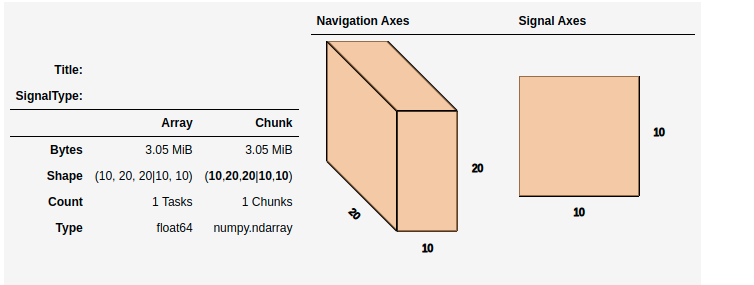
Computing lazy signals

Upon saving lazy signals, the result of computations is stored on disk.

In order to store the lazy signal in memory (i.e. make it a normal HyperSpy signal) it has a compute() method:

>>> s
<LazySignal2D, title: , dimensions: (10, 20, 20|10, 10)>
>>> s.compute()
[########################################] | 100% Completed |  0.1s
>>> s
<Signal2D, title: , dimensions: (10, 20, 20|10, 10)>

Lazy operations that affect the axes

When using lazy signals the computation of the data is delayed until requested. However, the changes to the axes properties are performed when running a given function that modfies them i.e. they are not performed lazily. This can lead to hard to debug issues when the result of a given function that is computed lazily depends on the value of the axes parameters that may have changed before the computation is requested. Therefore, in order to avoid such issues, it is reccomended to explicitly compute the result of all functions that are affected by the axes parameters. This is the reason why e.g. the result of shift1D() is not lazy.

Dask Scheduler

Dask is a flexible library for parallel computing in Python. All of the lazy operations (and many of the non lazy operations) in hyperspy run through dask. Dask can be used to run computations on a single machine or scaled to a cluster. This section introduces the different schedulers and how to use them in HyperSpy - for more details, see the dask documention on scheduling.

Note

To scale on multiple machines, e.g. a computer cluster, the distributed scheduler is required.

Single Threaded Scheduler

The single threaded scheduler in dask is useful for debugging and testing. It is not recommended for general use.

>>> import dask
>>> import hyperspy.api as hs
>>> import numpy as np
>>> import dask.array as da

Set the scheduler to single-threaded globally

>>> dask.config.set(scheduler='single-threaded')

Alternatively, you can set the scheduler to single-threaded for a single function call by setting the scheduler keyword argument to 'single-threaded'.

Or for something like plotting you can set the scheduler to single-threaded for the duration of the plotting call by using the with dask.config.set context manager.

>>> s.compute(scheduler="single-threaded")

>>> with dask.config.set(scheduler='single-threaded'):
...     s.plot()

Single Machine Schedulers

Dask has two schedulers available for single machines.

1. Threaded Scheduler:

   Fastest to set up but only provides parallelism through threads so only non python functions will be parallelized. This is good if you have largely numpy code and not too many cores.

2. Processes Scheduler:

   Each task (and all of the necessary dependencies) are shipped to different processes. As such it has a larger set up time. This preforms well for python dominated code.

>>> import dask
>>> dask.config.set(scheduler='processes')

Any hyperspy code will now use the multiprocessing scheduler

>>> s.compute()

Change to threaded Scheduler, overwrite default

>>> dask.config.set(scheduler='threads')
>>> s.compute()

Distributed Scheduler

Warning

Distributed computing is not supported for all file formats.

Distributed computing is limited to a few file formats, see the list of supported file format in RosettaSciIO documentation. If the format you are using is not supported, it is recommended to convert the file to zspy by reading with a single machine scheduler and saving it as a zspy file.

The recommended way to use dask is with the distributed scheduler. This allows you to scale your computations to a cluster of machines. The distributed scheduler can be used on a single machine as well. dask-distributed also gives you access to the dask dashboard which allows you to monitor your computations.

Some operations such as the matrix decomposition algorithms in hyperspy don’t currently work with the distributed scheduler.

>>> from dask.distributed import Client
>>> from dask.distributed import LocalCluster
>>> import dask.array as da
>>> import hyperspy.api as hs

>>> cluster = LocalCluster()
>>> client = Client(cluster)
>>> client

Any calculation will now use the distributed scheduler

>>> s
>>> s.plot()
>>> s.compute()

Running computation on remote cluster can be done easily using dask_jobqueue

>>> from dask_jobqueue import SLURMCluster
>>> from dask.distributed import Client
>>> cluster = SLURMCluster(cores=48,
...                        memory='120Gb',
...                        walltime="01:00:00",
...                        queue='research')

Get 3 nodes

>>> cluster.scale(jobs=3)
>>> client = Client(cluster)
>>> client

Any calculation will now use the distributed scheduler

>>> s = hs.data.two_gaussians()
>>> repeated_data = da.repeat(da.array(s.data[np.newaxis, :]),10, axis=0)
>>> s = hs.signals.Signal1D(repeated_data).as_lazy()
>>> summed = s.map(np.sum, inplace=False)
>>> s.compute()

Limitations

Most operations can be performed lazily. However, lazy operations come with a few limitations and constraints that we detail below.

Immutable signals

An important limitation when using LazySignal is the inability to modify existing data (immutability). This is a logical consequence of the DAG (tree structure, explained in Behind the scenes – technical details), where a complete history of the processing has to be stored to traverse later.

In fact, lazy evaluation removes the need for such operation, since only additional tree branches are added, requiring very little resources. In practical terms the following fails with lazy signals:

>>> s = hs.signals.BaseSignal([0]).as_lazy()
>>> s += 1
Traceback (most recent call last):
  File "<ipython-input-6-1bd1db4187be>", line 1, in <module>
    s += 1
  File "<string>", line 2, in __iadd__
  File "/home/fjd29/Python/hyperspy3/hyperspy/signal.py", line 1591, in _binary_operator_ruler
    getattr(self.data, op_name)(other)
AttributeError: 'Array' object has no attribute '__iadd__'

However, when operating lazily there is no clear benefit to using in-place operations. So, the operation above could be rewritten as follows:

>>> s = hs.signals.BaseSignal([0]).as_lazy()
>>> s = s + 1

Or even better:

>>> s = hs.signals.BaseSignal([0]).as_lazy()
>>> s1 = s + 1

Other minor differences

• Histograms for a LazySignal do not support knuth and blocks binning algorithms.

• CircleROI sets the elements outside the ROI to np.nan instead of using a masked array, because dask does not support masking. As a convenience, nansum, nanmean and other nan* signal methods were added to mimic the workflow as closely as possible.

Saving Big Data

The most efficient format supported by RosettaSciIO to write data is the ZSpy format, mainly because it supports writing concurrently from multiple threads or processes. This also allows for smooth interaction with dask-distributed for efficient scaling.

Behind the scenes – technical details

Standard HyperSpy signals load the data into memory for fast access and processing. While this behaviour gives good performance in terms of speed, it obviously requires at least as much computer memory as the dataset, and often twice that to store the results of subsequent computations. This can become a significant problem when processing very large datasets on consumer-oriented hardware.

HyperSpy offers a solution for this problem by including LazySignal and its derivatives. The main idea of these classes is to perform any operation (as the name suggests) lazily (delaying the execution until the result is requested (e.g. saved, plotted)) and in a blocked fashion. This is achieved by building a “history tree” (formally called a Directed Acyclic Graph (DAG)) of the computations, where the original data is at the root, and any further operations branch from it. Only when a certain branch result is requested, the way to the root is found and evaluated in the correct sequence on the correct blocks.

The “magic” is performed by (for the sake of simplicity) storing the data not as numpy.ndarray, but dask.array.Array (see the dask documentation). dask offers a couple of advantages:

• Arbitrary-sized data processing is possible. By only loading a couple of chunks at a time, theoretically any signal can be processed, albeit slower. In practice, this may be limited: (i) some operations may require certain chunking pattern, which may still saturate memory; (ii) many chunks should fit into the computer memory comfortably at the same time.

• Loading only the required data. If a certain part (chunk) of the data is not required for the final result, it will not be loaded at all, saving time and resources.

• Able to extend to a distributed computing environment (clusters). :dask.distributed (see the dask documentation) offers a straightforward way to expand the effective memory for computations to that of a cluster, which allows performing the operations significantly faster than on a single machine.