Generic tools#

Below we briefly introduce some of the most commonly used tools (methods). For more details about a particular method click on its name. For a detailed list of all the methods available see the BaseSignal documentation.

The methods of this section are available to all the signals. In other chapters methods that are only available in specialized subclasses are listed.

Mathematical operations#

A number of mathematical operations are available in BaseSignal. Most of them are just wrapped numpy functions.

The methods that perform mathematical operation over one or more axis at a time are:

Note that by default all this methods perform the operation over all navigation axes.

Example:

>>> s = hs.signals.BaseSignal(np.random.random((2,4,6)))
>>> s.axes_manager[0].name = 'E'
>>> s
<BaseSignal, title: , dimensions: (|6, 4, 2)>
>>> # by default perform operation over all navigation axes
>>> s.sum()
<BaseSignal, title: , dimensions: (|6, 4, 2)>
>>> # can also pass axes individually
>>> s.sum('E')
<Signal2D, title: , dimensions: (|4, 2)>
>>> # or a tuple of axes to operate on, with duplicates, by index or directly
>>> ans = s.sum((-1, s.axes_manager[1], 'E', 0))
>>> ans
<BaseSignal, title: , dimensions: (|1)>
>>> ans.axes_manager[0]
<Scalar axis, size: 1>

The following methods operate only on one axis at a time:

All numpy ufunc can operate on BaseSignal instances, for example:

>>> s = hs.signals.Signal1D([0, 1])
>>> s.metadata.General.title = "A"
>>> s
<Signal1D, title: A, dimensions: (|2)>
>>> np.exp(s)
<Signal1D, title: exp(A), dimensions: (|2)>
>>> np.exp(s).data
array([1. , 2.71828183])
>>> np.power(s, 2)
<Signal1D, title: power(A, 2), dimensions: (|2)>
>>> np.add(s, s)
<Signal1D, title: add(A, A), dimensions: (|2)>
>>> np.add(hs.signals.Signal1D([0, 1]), hs.signals.Signal1D([0, 1]))
<Signal1D, title: add(Untitled Signal 1, Untitled Signal 2), dimensions: (|2)>

Notice that the title is automatically updated. When the signal has no title a new title is automatically generated:

>>> np.add(hs.signals.Signal1D([0, 1]), hs.signals.Signal1D([0, 1]))
<Signal1D, title: add(Untitled Signal 1, Untitled Signal 2), dimensions: (|2)>

Functions (other than unfucs) that operate on numpy arrays can also operate on BaseSignal instances, however they return a numpy array instead of a BaseSignal instance e.g.:

>>> np.angle(s)
array([0., 0.])

Note

For numerical differentiation and integration, use the proper methods derivative() and integrate1D(). In certain cases, particularly when operating on a non-uniform axis, the approximations using the diff() and sum() methods will lead to erroneous results.

Signal operations#

BaseSignal supports all the Python binary arithmetic operations (+, -, *, //, %, divmod(), pow(), **, <<, >>, &, ^, |), augmented binary assignments (+=, -=, *=, /=, //=, %=, **=, <<=, >>=, &=, ^=, |=), unary operations (-, +, abs() and ~) and rich comparisons operations (<, <=, ==, x!=y, <>, >, >=).

These operations are performed element-wise. When the dimensions of the signals are not equal numpy broadcasting rules apply independently for the navigation and signal axes.

Warning

Hyperspy does not check if the calibration of the signals matches.

In the following example s2 has only one navigation axis while s has two. However, because the size of their first navigation axis is the same, their dimensions are compatible and s2 is broadcasted to match s’s dimensions.

>>> s = hs.signals.Signal2D(np.ones((3,2,5,4)))
>>> s2 = hs.signals.Signal2D(np.ones((2,5,4)))
>>> s
<Signal2D, title: , dimensions: (2, 3|4, 5)>
>>> s2
<Signal2D, title: , dimensions: (2|4, 5)>
>>> s + s2
<Signal2D, title: , dimensions: (2, 3|4, 5)>

In the following example the dimensions are not compatible and an exception is raised.

>>> s = hs.signals.Signal2D(np.ones((3,2,5,4)))
>>> s2 = hs.signals.Signal2D(np.ones((3,5,4)))
>>> s
<Signal2D, title: , dimensions: (2, 3|4, 5)>
>>> s2
<Signal2D, title: , dimensions: (3|4, 5)>
>>> s + s2 
Traceback (most recent call last):
  File "<ipython-input-55-044bb11a0bd9>", line 1, in <module>
    s + s2
  File "<string>", line 2, in __add__
  File "/home/fjd29/Python/hyperspy/hyperspy/signal.py", line 2686, in _binary_operator_ruler
    raise ValueError(exception_message)
ValueError: Invalid dimensions for this operation

Broadcasting operates exactly in the same way for the signal axes:

>>> s = hs.signals.Signal2D(np.ones((3,2,5,4)))
>>> s2 = hs.signals.Signal1D(np.ones((3, 2, 4)))
>>> s
<Signal2D, title: , dimensions: (2, 3|4, 5)>
>>> s2
<Signal1D, title: , dimensions: (2, 3|4)>
>>> s + s2
<Signal2D, title: , dimensions: (2, 3|4, 5)>

In-place operators also support broadcasting, but only when broadcasting would not change the left most signal dimensions:

>>> s += s2
>>> s
<Signal2D, title: , dimensions: (2, 3|4, 5)>
>>> s2 += s 
Traceback (most recent call last):
  File "<ipython-input-64-fdb9d3a69771>", line 1, in <module>
    s2 += s
  File "<string>", line 2, in __iadd__
  File "/home/fjd29/Python/hyperspy/hyperspy/signal.py", line 2737, in _binary_operator_ruler
    self.data = getattr(sdata, op_name)(odata)
ValueError: non-broadcastable output operand with shape (3,2,1,4) doesn\'t match the broadcast shape (3,2,5,4)

Iterating over the navigation axes#

BaseSignal instances are iterables over the navigation axes. For example, the following code creates a stack of 10 images and saves them in separate “png” files by iterating over the signal instance:

>>> image_stack = hs.signals.Signal2D(np.random.randint(10, size=(2, 5, 64,64)))
>>> for single_image in image_stack:
...    single_image.save("image %s.png" % str(image_stack.axes_manager.indices)) 
The "image (0, 0).png" file was created.
The "image (1, 0).png" file was created.
The "image (2, 0).png" file was created.
The "image (3, 0).png" file was created.
The "image (4, 0).png" file was created.
The "image (0, 1).png" file was created.
The "image (1, 1).png" file was created.
The "image (2, 1).png" file was created.
The "image (3, 1).png" file was created.
The "image (4, 1).png" file was created.

The data of the signal instance that is returned at each iteration is a view of the original data, a property that we can use to perform operations on the data. For example, the following code rotates the image at each coordinate by a given angle and uses the stack() function in combination with list comprehensions to make a horizontal “collage” of the image stack:

>>> import scipy.ndimage
>>> image_stack = hs.signals.Signal2D(np.array([scipy.datasets.ascent()]*5))
>>> image_stack.axes_manager[1].name = "x"
>>> image_stack.axes_manager[2].name = "y"
>>> for image, angle in zip(image_stack, (0, 45, 90, 135, 180)):
...    image.data[:] = scipy.ndimage.rotate(image.data, angle=angle,
...    reshape=False)
>>> # clip data to integer range:
>>> image_stack.data = np.clip(image_stack.data, 0, 255)
>>> collage = hs.stack([image for image in image_stack], axis=0)
>>> collage.plot(scalebar=False)

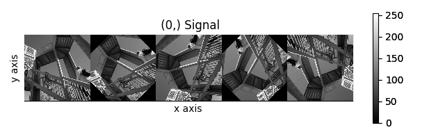
../../_images/rotate_ascent.png — Rotation of images by iteration.#

Iterating external functions with the map method#

Performing an operation on the data at each coordinate, as in the previous example, using an external function can be more easily accomplished using the map() method:

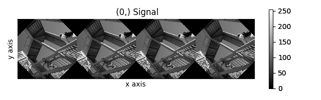
>>> import scipy.ndimage
>>> image_stack = hs.signals.Signal2D(np.array([scipy.datasets.ascent()]*4))
>>> image_stack.axes_manager[1].name = "x"
>>> image_stack.axes_manager[2].name = "y"
>>> image_stack.map(scipy.ndimage.rotate, angle=45, reshape=False)
>>> # clip data to integer range
>>> image_stack.data = np.clip(image_stack.data, 0, 255)
>>> collage = hs.stack([image for image in image_stack], axis=0)
>>> collage.plot()

../../_images/rotate_ascent_apply_simple.png — Rotation of images by the same amount using `map()`.#

The map() method can also take variable arguments as in the following example.

>>> import scipy.ndimage
>>> image_stack = hs.signals.Signal2D(np.array([scipy.datasets.ascent()]*4))
>>> image_stack.axes_manager[1].name = "x"
>>> image_stack.axes_manager[2].name = "y"
>>> angles = hs.signals.BaseSignal(np.array([0, 45, 90, 135]))
>>> image_stack.map(scipy.ndimage.rotate, angle=angles.T, reshape=False)

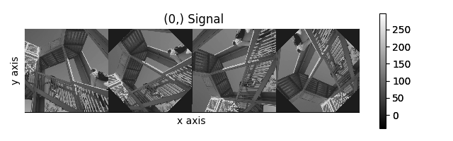
../../_images/rotate_ascent_apply_ndkwargs.png — Rotation of images using `map()` with different arguments for each image in the stack.#

New in version 1.2.0: inplace keyword and non-preserved output shapes

If all function calls do not return identically-shaped results, only navigation information is preserved, and the final result is an array where each element corresponds to the result of the function (or arbitrary object type). These are ragged arrays and has the dtype object. As such, most HyperSpy functions cannot operate on such signals, and the data should be accessed directly.

The inplace keyword (by default True) of the map() method allows either overwriting the current data (default, True) or storing it to a new signal (False).

>>> import scipy.ndimage
>>> image_stack = hs.signals.Signal2D(np.array([scipy.datasets.ascent()]*4))
>>> angles = hs.signals.BaseSignal(np.array([0, 45, 90, 135]))
>>> result = image_stack.map(scipy.ndimage.rotate,
...                            angle=angles.T,
...                            inplace=False,
...                            ragged=True,
...                            reshape=True)

>>> result
<BaseSignal, title: , dimensions: (4|ragged)>
>>> result.data.dtype
dtype('O')
>>> for d in result.data.flat:
...     print(d.shape)
(512, 512)
(724, 724)
(512, 512)
(724, 724)

New in version 1.4: Iterating over signal using a parameter with no navigation dimension.

In this case, the parameter is cyclically iterated over the navigation dimension of the input signal. In the example below, signal s is multiplied by a cosine parameter d, which is repeated over the navigation dimension of s.

>>> s = hs.signals.Signal1D(np.random.rand(10, 512))
>>> d = hs.signals.Signal1D(np.cos(np.linspace(0., 2*np.pi, 512)))
>>> s.map(lambda A, B: A * B, B=d)

New in version 1.7: Get result as lazy signal

Especially when working with very large datasets, it can be useful to not do the computation immediately. For example if it would make you run out of memory. In that case, the lazy_output parameter can be used.

>>> from scipy.ndimage import gaussian_filter
>>> s = hs.signals.Signal2D(np.random.random((4, 4, 128, 128)))
>>> s_out = s.map(gaussian_filter, sigma=5, inplace=False, lazy_output=True)
>>> s_out
<LazySignal2D, title: , dimensions: (4, 4|128, 128)>

s_out can then be saved to a hard drive, to avoid it being loaded into memory. Alternatively, it can be computed and loaded into memory using s_out.compute()

>>> s_out.save("gaussian_filter_file.hspy") 

Another advantage of using lazy_output=True is the ability to “chain” operations, by running map() on the output from a previous map() operation. For example, first running a Gaussian filter, followed by peak finding. This can improve the computation time, and reduce the memory need.

>>> s_out = s.map(scipy.ndimage.gaussian_filter, sigma=5, inplace=False, lazy_output=True)
>>> from skimage.feature import blob_dog
>>> s_out1 = s_out.map(blob_dog, threshold=0.05, inplace=False, ragged=True, lazy_output=False)
>>> s_out1
<BaseSignal, title: , dimensions: (4, 4|ragged)>

This is especially relevant for very large datasets, where memory use can be a limiting factor.

Cropping#

Cropping can be performed in a very compact and powerful way using Indexing . In addition it can be performed using the following method or GUIs if cropping signal1D or signal2D. There is also a general crop() method that operates in place.

Rebinning#

New in version 1.3: rebin() generalized to remove the constrain of the new_shape needing to be a divisor of data.shape.

The rebin() methods supports rebinning the data to arbitrary new shapes as long as the number of dimensions stays the same. However, internally, it uses two different algorithms to perform the task. Only when the new shape dimensions are divisors of the old shape’s, the operation supports lazy-evaluation and is usually faster. Otherwise, the operation requires linear interpolation.

For example, the following two equivalent rebinning operations can be performed lazily:

>>> s = hs.data.two_gaussians().as_lazy()
>>> print(s)
<LazySignal1D, title: Two Gaussians, dimensions: (32, 32|1024)>
>>> print(s.rebin(scale=[1, 1, 2]))
<LazySignal1D, title: Two Gaussians, dimensions: (32, 32|512)>

>>> s = hs.data.two_gaussians().as_lazy()
>>> print(s.rebin(new_shape=[32, 32, 512]))
<LazySignal1D, title: Two Gaussians, dimensions: (32, 32|512)>

On the other hand, the following rebinning operation requires interpolation and cannot be performed lazily:

>>> s = hs.signals.Signal1D(np.ones([4, 4, 10]))
>>> s.data[1, 2, 9] = 5
>>> print(s)
<Signal1D, title: , dimensions: (4, 4|10)>
>>> print ('Sum = ', s.data.sum())
Sum =  164.0
>>> scale = [0.5, 0.5, 5]
>>> test = s.rebin(scale=scale)
>>> test2 = s.rebin(new_shape=(8, 8, 2)) # Equivalent to the above
>>> print(test)
<Signal1D, title: , dimensions: (8, 8|2)>
>>> print(test2)
<Signal1D, title: , dimensions: (8, 8|2)>
>>> print('Sum =', test.data.sum())
Sum = 164.0
>>> print('Sum =', test2.data.sum())
Sum = 164.0
>>> s.as_lazy().rebin(scale=scale) 
Traceback (most recent call last):
  File "<ipython-input-26-49bca19ebf34>", line 1, in <module>
    spectrum.as_lazy().rebin(scale=scale)
  File "/home/fjd29/Python/hyperspy3/hyperspy/_signals/eds.py", line 184, in rebin
    m = super().rebin(new_shape=new_shape, scale=scale, crop=crop, out=out)
  File "/home/fjd29/Python/hyperspy3/hyperspy/_signals/lazy.py", line 246, in rebin
    "Lazy rebin requires scale to be integer and divisor of the "
NotImplementedError: Lazy rebin requires scale to be integer and divisor of the original signal shape

The dtype argument can be used to specify the dtype of the returned signal:

>>> s = hs.signals.Signal1D(np.ones((2, 5, 10), dtype=np.uint8))
>>> print(s)
<Signal1D, title: , dimensions: (5, 2|10)>
>>> print(s.data.dtype)
uint8

Use dtype=np.unit16 to specify a dtype:

>>> s2 = s.rebin(scale=(5, 2, 1), dtype=np.uint16)
>>> print(s2.data.dtype)
uint16

Use dtype="same" to keep the same dtype:

>>> s3 = s.rebin(scale=(5, 2, 1), dtype="same")
>>> print(s3.data.dtype)
uint8

By default dtype=None, the dtype is determined by the behaviour of numpy.sum, in this case, unsigned integer of the same precision as the platform interger:

>>> s4 = s.rebin(scale=(5, 2, 1))
>>> print(s4.data.dtype)
uint32

Interpolate to a different axis#

The interpolate_on_axis() method makes it possible to exchange any existing axis of a signal with a new axis, regardless of the signals dimension or the axes types. This is achieved by interpolating the data using scipy.interpolate.make_interp_spline() from the old axis to the new axis. Replacing multiple axes can be done iteratively.

>>> from hyperspy.axes import UniformDataAxis, DataAxis
>>> x = {"offset": 0, "scale": 1, "size": 10, "name": "X", "navigate": True}
>>> e = {"offset": 0, "scale": 1, "size": 50, "name": "E", "navigate": False}
>>> s = hs.signals.Signal1D(np.random.random((10, 50)), axes=[x, e])
>>> s
<Signal1D, title: , dimensions: (10|50)>
>>> x_new = UniformDataAxis(offset=1.5, scale=0.8, size=7, name="X_NEW", navigate=True)
>>> e_new = DataAxis(axis=np.arange(8)**2, name="E_NEW", navigate=False)
>>> s2 = s.interpolate_on_axis(x_new, 0, inplace=False)
>>> s2
<Signal1D, title: , dimensions: (7|50)>
>>> s2.interpolate_on_axis(e_new, "E", inplace=True)
>>> s2
<Signal1D, title: , dimensions: (7|8)>

Squeezing#

The squeeze() method removes any zero-dimensional axes, i.e. axes of size=1, and the attributed data dimensions from a signal. The method returns a reduced copy of the signal and does not operate in place.

>>> s = hs.signals.Signal2D(np.random.random((2, 1, 1, 6, 8, 8)))
>>> s
<Signal2D, title: , dimensions: (6, 1, 1, 2|8, 8)>
>>> s = s.squeeze()
>>> s
<Signal2D, title: , dimensions: (6, 2|8, 8)>

Squeezing can be particularly useful after a rebinning operation that leaves one dimension with shape=1:

>>> s = hs.signals.Signal2D(np.random.random((5,5,5,10,10)))
>>> s.rebin(new_shape=(5,1,5,5,5))
<Signal2D, title: , dimensions: (5, 1, 5|5, 5)>
>>> s.rebin(new_shape=(5,1,5,5,5)).squeeze()
<Signal2D, title: , dimensions: (5, 5|5, 5)>

Folding and unfolding#

When dealing with multidimensional datasets it is sometimes useful to transform the data into a two dimensional dataset. This can be accomplished using the following two methods:

It is also possible to unfold only the navigation or only the signal space:

Splitting and stacking#

Several objects can be stacked together over an existing axis or over a new axis using the stack() function, if they share axis with same dimension.

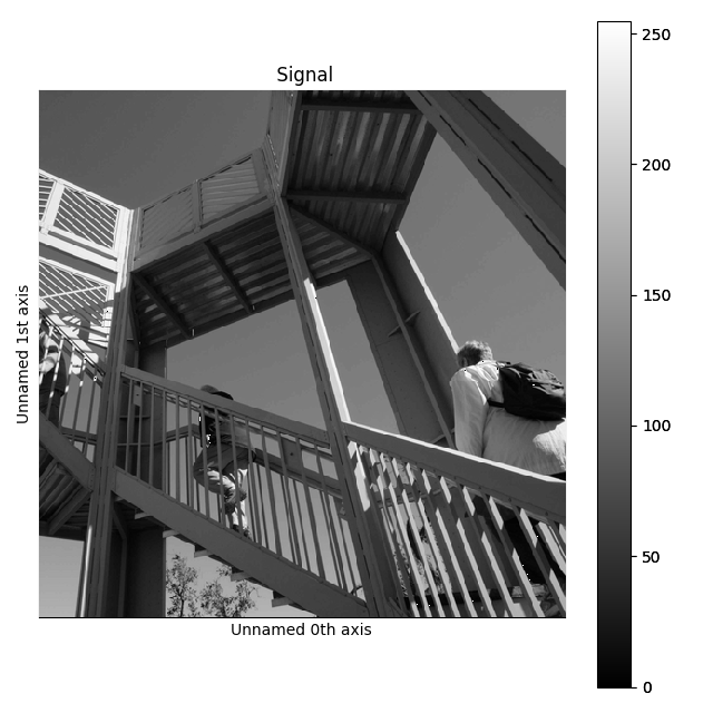
>>> image = hs.signals.Signal2D(scipy.datasets.ascent())
>>> image = hs.stack([hs.stack([image]*3,axis=0)]*3,axis=1)
>>> image.plot()

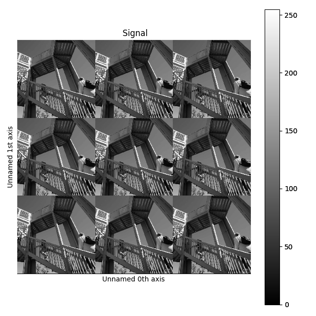
../../_images/stack_ascent_3_3.png — Stacking example.#

Note

When stacking signals with large amount of original_metadata, these metadata will be stacked and this can lead to very large amount of metadata which can in turn slow down processing. The stack_original_metadata argument can be used to disable stacking original_metadata.

An object can be split into several objects with the split() method. This function can be used to reverse the stack() function:

>>> image = image.split()[0].split()[0]
>>> image.plot()

../../_images/split_ascent_3_3.png — Splitting example.#

Fast Fourier Transform (FFT)#

The fast Fourier transform of a signal can be computed using the fft() method. By default, the FFT is calculated with the origin at (0, 0), which will be displayed at the bottom left and not in the centre of the FFT. Conveniently, the shift argument of the the fft() method can be used to center the output of the FFT. In the following example, the FFT of a hologram is computed using shift=True and its output signal is displayed, which shows that the FFT results in a complex signal with a real and an imaginary parts:

>>> im = hs.data.wave_image()
>>> fft_shifted = im.fft(shift=True)
>>> fft_shifted.plot()

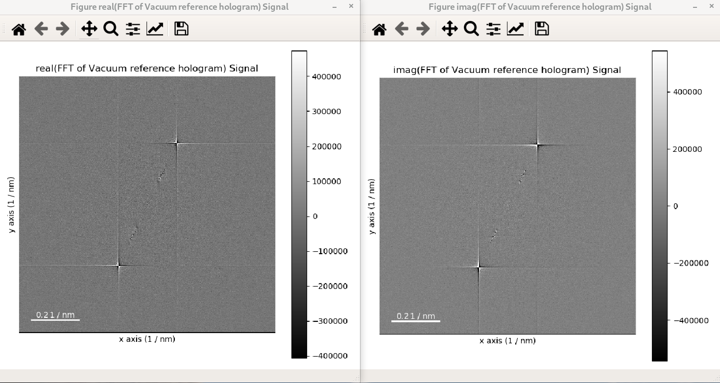
../../_images/FFT_vacuum_reference_hologram.png

The strong features in the real and imaginary parts correspond to the lattice fringes of the hologram.

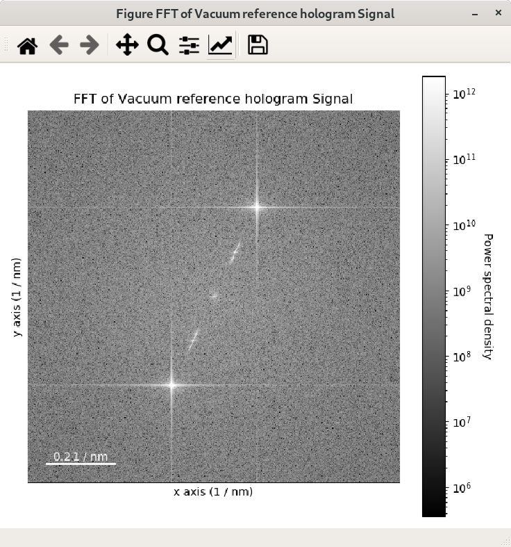
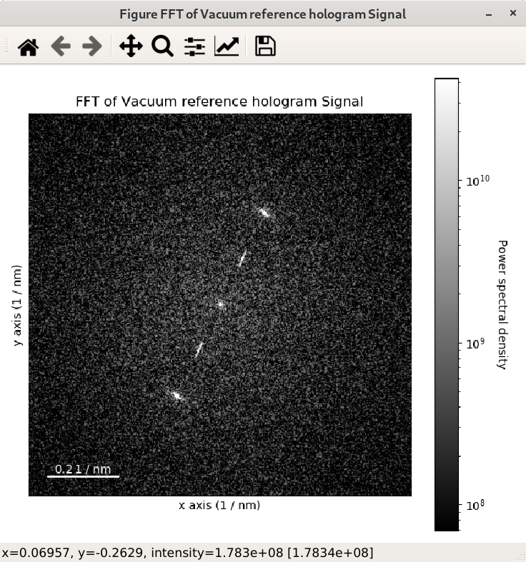
For visual inspection of the FFT it is convenient to display its power spectrum (i.e. the square of the absolute value of the FFT) rather than FFT itself as it is done in the example above by using the power_spectum argument:

>>> im = hs.data.wave_image()
>>> fft = im.fft(True)
>>> fft.plot(True)

Where power_spectum is set to True since it is the first argument of the plot() method for complex signal. When power_spectrum=True, the plot will be displayed on a log scale by default.

../../_images/FFT_vacuum_reference_hologram_power_spectrum.png

The visualisation can be further improved by setting the minimum value to display to the 30-th percentile; this can be done by using vmin="30th" in the plot function:

>>> im = hs.data.wave_image()
>>> fft = im.fft(True)
>>> fft.plot(True, vmin="30th")

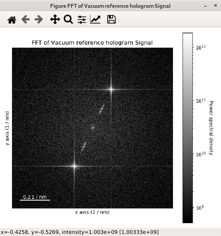
../../_images/FFT_vacuum_reference_hologram_power_spectrum_vmin30th.png

The streaks visible in the FFT come from the edge of the image and can be removed by applying an apodization function to the original signal before the computation of the FFT. This can be done using the apodization argument of the fft() method and it is usually used for visualising FFT patterns rather than for quantitative analyses. By default, the so-called hann windows is used but different type of windows such as the hamming and tukey windows.

>>> im = hs.data.wave_image()
>>> fft = im.fft(shift=True)
>>> fft_apodized = im.fft(shift=True, apodization=True)
>>> fft_apodized.plot(True, vmin="30th")

../../_images/FFT_vacuum_reference_hologram_power_spectrum_vmin30th-apodization.png

Inverse Fast Fourier Transform (iFFT)#

Inverse fast Fourier transform can be calculated from a complex signal by using the ifft() method. Similarly to the fft() method, the shift argument can be provided to shift the origin of the iFFT when necessary:

>>> im_ifft = im.fft(shift=True).ifft(shift=True)

Changing the data type#

Even if the original data is recorded with a limited dynamic range, it is often desirable to perform the analysis operations with a higher precision. Conversely, if space is limited, storing in a shorter data type can decrease the file size. The change_dtype() changes the data type in place, e.g.:

>>> s = hs.load('EELS Signal1D Signal2D (high-loss).dm3') 
    Title: EELS Signal1D Signal2D (high-loss).dm3
    Signal type: EELS
    Data dimensions: (21, 42, 2048)
    Data representation: spectrum
    Data type: float32
>>> s.change_dtype('float64') 
>>> print(s) 
    Title: EELS Signal1D Signal2D (high-loss).dm3
    Signal type: EELS
    Data dimensions: (21, 42, 2048)
    Data representation: spectrum
    Data type: float64

In addition to all standard numpy dtypes, HyperSpy supports four extra dtypes for RGB images for visualization purposes only: rgb8, rgba8, rgb16 and rgba16. This includes of course multi-dimensional RGB images.

The requirements for changing from and to any rgbx dtype are more strict than for most other dtype conversions. To change to a rgbx dtype the signal_dimension must be 1 and its size 3 (4) 3(4) for rgb (or rgba) dtypes and the dtype must be uint8 (uint16) for rgbx8 (rgbx16). After conversion the signal_dimension becomes 2.

Most operations on signals with RGB dtypes will fail. For processing simply change their dtype to uint8 (uint16).The dtype of images of dtype rgbx8 (rgbx16) can only be changed to uint8 (uint16) and the signal_dimension becomes 1.

In the following example we create a 1D signal with signal size 3 and with dtype uint16 and change its dtype to rgb16 for plotting.

>>> rgb_test = np.zeros((1024, 1024, 3))
>>> ly, lx = rgb_test.shape[:2]
>>> offset_factor = 0.16
>>> size_factor = 3
>>> Y, X = np.ogrid[0:lx, 0:ly]
>>> rgb_test[:,:,0] = (X - lx / 2 - lx*offset_factor) ** 2 + \
...                   (Y - ly / 2 - ly*offset_factor) ** 2 < \
...                   lx * ly / size_factor **2
>>> rgb_test[:,:,1] = (X - lx / 2 + lx*offset_factor) ** 2 + \
...                   (Y - ly / 2 - ly*offset_factor) ** 2 < \
...                   lx * ly / size_factor **2
>>> rgb_test[:,:,2] = (X - lx / 2) ** 2 + \
...                   (Y - ly / 2 + ly*offset_factor) ** 2 \
...                   < lx * ly / size_factor **2
>>> rgb_test *= 2**16 - 1
>>> s = hs.signals.Signal1D(rgb_test)
>>> s.change_dtype("uint16")
>>> s
<Signal1D, title: , dimensions: (1024, 1024|3)>
>>> s.change_dtype("rgb16")
>>> s
<Signal2D, title: , dimensions: (|1024, 1024)>
>>> s.plot()

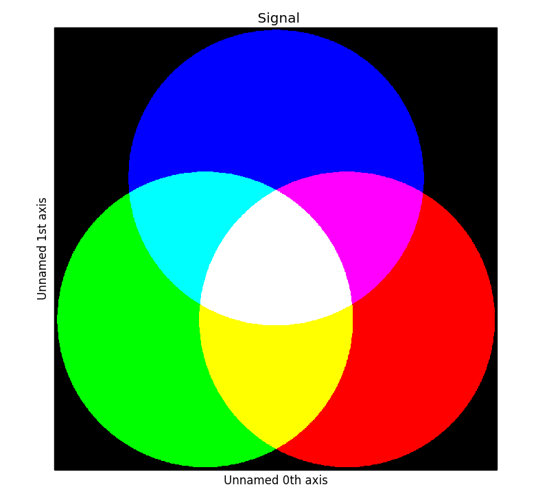
../../_images/rgb_example.png — RGB data type example.#

Transposing (changing signal spaces)#

New in version 1.1.

transpose() method changes how the dataset dimensions are interpreted (as signal or navigation axes). By default is swaps the signal and navigation axes. For example:

>>> s = hs.signals.Signal1D(np.zeros((4,5,6)))
>>> s
<Signal1D, title: , dimensions: (5, 4|6)>
>>> s.transpose()
<Signal2D, title: , dimensions: (6|5, 4)>

For T() is a shortcut for the default behaviour:

>>> s = hs.signals.Signal1D(np.zeros((4,5,6))).T
>>> s
<Signal2D, title: , dimensions: (6|5, 4)>

The method accepts both explicit axes to keep in either space, or just a number of axes required in one space (just one number can be specified, as the other is defined as “all other axes”). When axes order is not explicitly defined, they are “rolled” from one space to the other as if the <navigation axes | signal axes > wrap a circle. The example below should help clarifying this.

>>> # just create a signal with many distinct dimensions
>>> s = hs.signals.BaseSignal(np.random.rand(1, 2, 3, 4, 5, 6, 7, 8, 9))
>>> s
<BaseSignal, title: , dimensions: (|9, 8, 7, 6, 5, 4, 3, 2, 1)>
>>> s.transpose(signal_axes=5) # roll to leave 5 axes in signal space
<BaseSignal, title: , dimensions: (4, 3, 2, 1|9, 8, 7, 6, 5)>
>>> s.transpose(navigation_axes=3) # roll leave 3 axes in navigation space
<BaseSignal, title: , dimensions: (3, 2, 1|9, 8, 7, 6, 5, 4)>
>>> # 3 explicitly defined axes in signal space
>>> s.transpose(signal_axes=[0, 2, 6])
<BaseSignal, title: , dimensions: (8, 6, 5, 4, 2, 1|9, 7, 3)>
>>> # A mix of two lists, but specifying all axes explicitly
>>> # The order of axes is preserved in both lists
>>> s.transpose(navigation_axes=[1, 2, 3, 4, 5, 8], signal_axes=[0, 6, 7])
<BaseSignal, title: , dimensions: (8, 7, 6, 5, 4, 1|9, 3, 2)>

A convenience functions transpose() is available to operate on many signals at once, for example enabling plotting any-dimension signals trivially:

>>> s2 = hs.signals.BaseSignal(np.random.rand(2, 2)) # 2D signal
>>> s3 = hs.signals.BaseSignal(np.random.rand(3, 3, 3)) # 3D signal
>>> s4 = hs.signals.BaseSignal(np.random.rand(4, 4, 4, 4)) # 4D signal
>>> hs.plot.plot_images(hs.transpose(s2, s3, s4, signal_axes=2)) 

The transpose() method accepts keyword argument optimize, which is False by default, meaning modifying the output signal data always modifies the original data i.e. the data is just a view of the original data. If True, the method ensures the data in memory is stored in the most efficient manner for iterating by making a copy of the data if required, hence modifying the output signal data not always modifies the original data.

The convenience methods as_signal1D() and as_signal2D() internally use transpose(), but always optimize the data for iteration over the navigation axes if required. Hence, these methods do not always return a view of the original data. If a copy of the data is required use deepcopy() on the output of any of these methods e.g.:

>>> hs.signals.Signal1D(np.zeros((4,5,6))).T.deepcopy()
<Signal2D, title: , dimensions: (6|5, 4)>

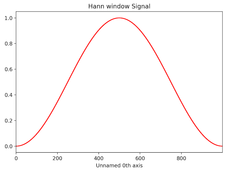
Applying apodization window#

Apodization window (also known as apodization function) can be applied to a signal using apply_apodization() method. By default standard Hann window is used:

>>> s = hs.signals.Signal1D(np.ones(1000))
>>> sa = s.apply_apodization()
>>> sa.metadata.General.title = 'Hann window'
>>> sa.plot()

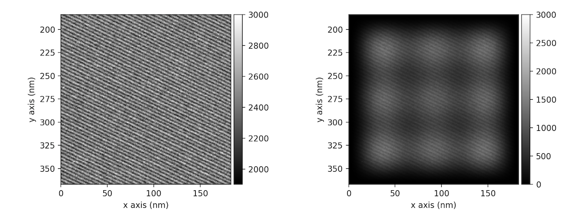
Higher order Hann window can be used in order to keep larger fraction of intensity of original signal. This can be done providing an integer number for the order of the window through keyword argument hann_order. (The last one works only together with default value of window argument or with window='hann'.)

>>> im = hs.data.wave_image().isig[:200, :200]
>>> ima = im.apply_apodization(window='hann', hann_order=3)
>>> hs.plot.plot_images([im, ima], vmax=3000, tight_layout=True)
[<Axes: >, <Axes: >]

../../_images/hann_3d_order_ref_holo.png

In addition to Hann window also Hamming or Tukey windows can be applied using window attribute selecting 'hamming' or 'tukey' respectively.

The shape of Tukey window can be adjusted using parameter alpha provided through tukey_alpha keyword argument (only used when window='tukey'). The parameter represents the fraction of the window inside the cosine tapered region, i.e. smaller is alpha larger is the middle flat region where the original signal is preserved. If alpha is one, the Tukey window is equivalent to a Hann window. (Default value is 0.5)

Apodization can be applied in place by setting keyword argument inplace to True. In this case method will not return anything.