Basic Usage#
Starting Python in Windows#
If you used the bundle installation you should be able to use the context menus to get started. Right-click on the folder containing the data you wish to analyse and select “Jupyter notebook here” or “Jupyter qtconsole here”. We recommend the former, since notebooks have many advantages over conventional consoles, as will be illustrated in later sections. The examples in some later sections assume Notebook operation. A new tab should appear in your default browser listing the files in the selected folder. To start a python notebook choose “Python 3” in the “New” drop-down menu at the top right of the page. Another new tab will open which is your Notebook.
Starting Python in Linux and MacOS#
You can start IPython by opening a system terminal and executing ipython,
(optionally followed by the “frontend”: “qtconsole” for example). However, in
most cases, the most agreeable way to work with HyperSpy interactively
is using the Jupyter Notebook (previously known as
the IPython Notebook), which can be started as follows:
$ jupyter notebook
Linux users may find it more convenient to start Jupyter/IPython from the file manager context menu. In either OS you can also start by double-clicking a notebook file if one already exists.
Starting HyperSpy in the notebook (or terminal)#
Typically you will need to set up IPython for interactive plotting with
matplotlib using
%matplotlib (which is known as a ‘Jupyter magic’)
before executing any plotting command. So, typically, after starting
IPython, you can import HyperSpy and set up interactive matplotlib plotting by
executing the following two lines in the IPython terminal (In these docs we
normally use the general Python prompt symbol >>> but you will probably
see In [1]: etc.):
>>> %matplotlib qt
>>> import hyperspy.api as hs
Note that to execute lines of code in the notebook you must press
Shift+Return. (For details about notebooks and their functionality try
the help menu in the notebook). Next, import two useful modules: numpy and
matplotlib.pyplot, as follows:
>>> import numpy as np
>>> import matplotlib.pyplot as plt
The rest of the documentation will assume you have done this. It also assumes that you have installed at least one of HyperSpy’s GUI packages: jupyter widgets GUI and the traitsui GUI.
Possible warnings when importing HyperSpy?#
HyperSpy supports different GUIs and matplotlib backends which in specific cases can lead to warnings when importing HyperSpy. Most of the time there is nothing to worry about — the warnings simply inform you of several choices you have. There may be several causes for a warning, for example:
not all the GUIs packages are installed. If none is installed, we reccomend you to install at least the
hyperspy-gui-ipywidgetspackage is your are planning to perform interactive data analysis in the Jupyter Notebook. Otherwise, you can simply disable the warning in preferences as explained below.the
hyperspy-gui-traitsuipackage is installed and you are using an incompatible matplotlib backend (e.g.notebook,nbaggorwidget).If you want to use the traitsui GUI, use the
qtmatplotlib backend instead.Alternatively, if you prefer to use the
notebookorwidgetmatplotlib backend, and if you don’t want to see the (harmless) warning, make sure that you have thehyperspy-gui-ipywidgetsinstalled and disable the traitsui GUI in the preferences.
Changed in version v1.3: HyperSpy works with all matplotlib backends, including the notebook
(also called nbAgg) backend that enables interactive plotting embedded
in the jupyter notebook.
Note
When running in a headless system it is necessary to set the matplotlib backend appropiately to avoid a cannot connect to X server error, for example as follows:
>>> import matplotlib
>>> matplotlib.rcParams["backend"] = "Agg"
>>> import hyperspy.api as hs
Getting help#
When using IPython, the documentation (docstring in Python jargon) can be accessed by adding a question mark to the name of a function. e.g.:
In [1]: import hyperspy.api as hs
This syntax is a shortcut to the standard way one of displaying the help associated to a given functions (docstring in Python jargon) and it is one of the many features of IPython, which is the interactive python shell that HyperSpy uses under the hood.
Autocompletion#
Another useful IPython feature is the autocompletion of commands and filenames using the tab and arrow keys. It is highly recommended to read the Ipython introduction for many more useful features that will boost your efficiency when working with HyperSpy/Python interactively.
Creating signal from a numpy array#
HyperSpy can operate on any numpy array by assigning it to a BaseSignal class.
This is useful e.g. for loading data stored in a format that is not yet
supported by HyperSpy—supposing that they can be read with another Python
library—or to explore numpy arrays generated by other Python
libraries. Simply select the most appropriate signal from the
signals module and create a new instance by passing a numpy array
to the constructor e.g.
>>> my_np_array = np.random.random((10, 20, 100))
>>> s = hs.signals.Signal1D(my_np_array)
>>> s
<Signal1D, title: , dimensions: (20, 10|100)>
The numpy array is stored in the data attribute
of the signal class:
>>> s.data
Saving Files#
The data can be saved to several file formats. The format is specified by the extension of the filename.
>>> # load the data
>>> d = hs.load("example.tif")
>>> # save the data as a tiff
>>> d.save("example_processed.tif")
>>> # save the data as a png
>>> d.save("example_processed.png")
>>> # save the data as an hspy file
>>> d.save("example_processed.hspy")
Some file formats are much better at maintaining the information about how you processed your data. The preferred formats are hspy and zspy, because they are open formats and keep most information possible.
There are optional flags that may be passed to the save function. See Saving for more details.
Accessing and setting the metadata#
When loading a file HyperSpy stores all metadata in the BaseSignal
original_metadata attribute. In addition,
some of those metadata and any new metadata generated by HyperSpy are stored in
metadata attribute.
>>> import exspy
>>> s = exspy.data.eelsdb(formula="NbO2", edge="M2,3")[0]
>>> s.metadata
├── Acquisition_instrument
│   └── TEM
│       ├── Detector
│       │   └── EELS
│       │       └── collection_angle = 6.5
│       ├── beam_energy = 100.0
│       ├── convergence_angle = 10.0
│       └── microscope = VG HB501UX
├── General
│   ├── author = Wilfried Sigle
│   └── title = Niobium oxide NbO2
├── Sample
│   ├── chemical_formula = NbO2
│   ├── description =  Analyst: David Bach, Wilfried Sigle. Temperature: Room.
│   └── elements = ['Nb', 'O']
└── Signal
    ├── quantity = Electrons ()
    └── signal_type = EELS

>>> s.original_metadata
├── emsa
│   ├── DATATYPE = XY
│   ├── DATE =
│   ├── FORMAT = EMSA/MAS Spectral Data File
│   ├── NCOLUMNS = 1.0
│   ├── NPOINTS = 1340.0
│   ├── OFFSET = 120.0003
│   ├── OWNER = eelsdatabase.net
│   ├── SIGNALTYPE = ELS
│   ├── TIME =
│   ├── TITLE = NbO2_Nb_M_David_Bach,_Wilfried_Sigle_217
│   ├── VERSION = 1.0
│   ├── XPERCHAN = 0.5
│   ├── XUNITS = eV
│   └── YUNITS =
└── json
    ├── api_permalink = https://api.eelsdb.eu/spectra/niobium-oxide-nbo2-2/
    ├── associated_spectra = [{'name': 'Niobium oxide NbO2', 'link': 'https://eelsdb.eu/spectra/niobium-oxide-nbo2/', 'type': 'Low Loss'}]
    ├── author
    │   ├── name = Wilfried Sigle
    │   ├── profile_api_url = https://api.eelsdb.eu/author/wsigle/
    │   └── profile_url = https://eelsdb.eu/author/wsigle/
    ├── beamenergy = 100 kV
    ├── collection = 6.5 mrad
    ├── comment_count = 0
    ├── convergence = 10 mrad
    ├── darkcurrent = Yes
    ├── description =  Analyst: David Bach, Wilfried Sigle. Temperature: Room.
    ├── detector = Parallel: Gatan ENFINA
    ├── download_link = https://eelsdb.eu/wp-content/uploads/2015/09/DspecYB7EbW.msa
    ├── edges = ['Nb_M2,3', 'Nb_M4,5', 'O_K']
    ├── elements = ['Nb', 'O']
    ├── formula = NbO2
    ├── gainvariation = Yes
    ├── guntype = cold field emission
    ├── id = 21727
    ├── integratetime = 5 secs
    ├── keywords = ['imported from old site']
    ├── max_energy = 789.5 eV
    ├── microscope = VG HB501UX
    ├── min_energy = 120 eV
    ├── monochromated = No
    ├── other_links = [{'url': 'http://pc-web.cemes.fr/eelsdb/index.php?page=displayspec.php&id=217', 'title': 'Old EELS DB'}]
    ├── permalink = https://eelsdb.eu/spectra/niobium-oxide-nbo2-2/
    ├── published = 2008-02-15 00:00:00
    ├── readouts = 10
    ├── resolution = 1.3 eV
    ├── stepSize = 0.5 eV/pixel
    ├── thickness = 0.58 t/λ
    ├── title = Niobium oxide NbO2
    └── type = Core Loss

>>> s.metadata.General.title = "NbO2 Nb_M edge"
>>> s.metadata
├── Acquisition_instrument
│   └── TEM
│       ├── Detector
│       │   └── EELS
│       │       └── collection_angle = 6.5
│       ├── beam_energy = 100.0
│       ├── convergence_angle = 10.0
│       └── microscope = VG HB501UX
├── General
│   ├── author = Wilfried Sigle
│   └── title = NbO2 Nb_M edge
├── Sample
│   ├── chemical_formula = NbO2
│   ├── description =  Analyst: David Bach, Wilfried Sigle. Temperature: Room.
│   └── elements = ['Nb', 'O']
└── Signal
    ├── quantity = Electrons ()
    └── signal_type = EELS
Configuring HyperSpy#
The behaviour of HyperSpy can be customised using the
preferences. The easiest way to do it is by calling
the gui() method:
>>> hs.preferences.gui()
This command should raise the Preferences user interface if one of the hyperspy gui packages are installed and enabled:
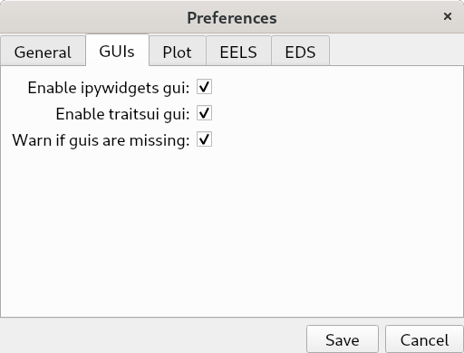
Preferences user interface.#
New in version 1.3: Possibility to enable/disable GUIs in the preferences.
It is also possible to set the preferences programmatically. For example, to disable the traitsui GUI elements and save the changes to disk:
>>> hs.preferences.GUIs.enable_traitsui_gui = False
>>> hs.preferences.save()
>>> # if not saved, this setting will be used until the next jupyter kernel shutdown
Changed in version 1.3: The following items were removed from preferences:
General.default_export_format, General.lazy,
Model.default_fitter, Machine_learning.multiple_files,
Machine_learning.same_window, Plot.default_style_to_compare_spectra,
Plot.plot_on_load, Plot.pylab_inline, EELS.fine_structure_width,
EELS.fine_structure_active, EELS.fine_structure_smoothing,
EELS.synchronize_cl_with_ll, EELS.preedge_safe_window_width,
EELS.min_distance_between_edges_for_fine_structure.
Messages log#
HyperSpy writes messages to the Python logger. The
default log level is “WARNING”, meaning that only warnings and more severe
event messages will be displayed. The default can be set in the
preferences. Alternatively, it can be set
using set_log_level() e.g.:
>>> import hyperspy.api as hs
>>> hs.set_log_level('INFO')
>>> hs.load('my_file.dm3')
INFO:hyperspy.io_plugins.digital_micrograph:DM version: 3
INFO:hyperspy.io_plugins.digital_micrograph:size 4796607 B
INFO:hyperspy.io_plugins.digital_micrograph:Is file Little endian? True
INFO:hyperspy.io_plugins.digital_micrograph:Total tags in root group: 15
<Signal2D, title: My file, dimensions: (|1024, 1024)